
In preparation for starting a new job next week, I’ve been doing some reading about neural networks and deep learning. The math behind neural networks is pretty interesting, so I thought I’d take my notes, and turn them into some posts.
As the name suggests, the basic idea of a neural network is to construct a computational system based on a simple model of a neuron. If you look at a neuron under a microscope, what you see is something vaguely similar to:
It’s a cell with three main parts:
- A central body;
- A collection of branched fibers called dendrites that receive signals and carry them to the body; and
- A branched fiber called an axon that sends signals produced by the body.
You can think of a neuron as a sort of analog computing element. Its dendrites receive inputs from some collection of sources. The body has some criteria for deciding, based on its inputs, whether to “fire”. If it fires, it sends an output using its axon.
What makes a neuron fire? It’s a combination of inputs. Different terminals on the dendrites have different signaling strength. When the combined inputs reach a threshold, the neuron fires. Those different signal strengths are key: a system of neurons can learn how to interpret a complex signal by varying the strength of the signal from different dendrites.
We can think of this simple model of a neuron in computational terms as a computing element that takes a set of weighted input values, combines them into a single value, and then generates an output of “1” if that value exceeds a threshold, and 0 if it does not.
In slightly more formal terms, ")
-
is the number of inputs to the machine. We’ll represent a given input as a vector
.
-
is a vector of weights, where
is the weight for input
.
-
is a bias value.
-
is the threshold for firing.
Given an input vector 

![v \cdot w = [\theta_1v_1 + \theta_2v_2 + ... + \theta_nv_n]](http://l.wordpress.com/latex.php?latex=v%20%5Ccdot%20w%20%3D%20%5B%5Ctheta_1v_1%20%2B%20%5Ctheta_2v_2%20%2B%20...%20%2B%20%5Ctheta_nv_n%5D&bg=FFFFFF&fg=000000&s=0 "v \cdot w = [\theta_1v_1 + \theta_2v_2 + ... + \theta_nv_n]")

This version of a neuron is called a perceptron. It’s good at a particular kind of task called classification: given a set of inputs, it can answer whether or not the input is a member of a particular subset of values. A simple perceptron is limited to linear classification, which I’ll explain next.
To understand what a perceptron does, the easiest way to think of it is graphical. Imagine you’ve got an input vector with two values, so that your inputs are points in a two dimensional cartesian plane. The weights on the perceptron inputs define a line in that plane. The perceptron fires for all points above that line – so the perceptron classifies a point according to which side of the line it’s located on. We can generalize that notion to higher dimensional spaces: for a perceptron taking
Taken by itself, a single perceptron isn’t very interesting. It’s just a fancy name for a something that implements a linear partition. What starts to unlock its potential is training. You can take a perceptron and initialize all of its weights to 1, and then start testing it on some input data. Based on the results of the tests, you alter the weights. After enough cycles of repeating this, the perceptron can learn the correct weights for any linear classification.
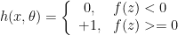
The traditional representation of the perceptron is as a function 

Using this model, learning is just an optimization process, where we’re trying to find a set of values for 
A linear perceptron is a implementation of this model based on a very simple notion of a neuron. A perceptron takes a set of weighted inputs, adds them together, and then if the result exceeds some threshold, it “fires”.
A perceptron whose weighted inputs don’t exceed its threshold produces an output of 0; a perceptron which “fires” based on its inputs produces a value of +1.
Linear classification is very limited – we’d like to be able to do things that are more interesting that just linear. We can do that by adding one thing to our definition of a neuron: an activation function. Instead of just checking if the value exceeds a threshold, we can take the dot-product of the inputs, and then apply a function to them before comparing them to the threshold.
With an activation function 
The logit is defined as:
 + b")
And the perceptron as a whole is a classifier:
Like I said before, this gets interesting when you get to the point of training. The idea is that before you start training, you have a neuron that doesn’t know anything about the things it’s trying to classify. You take a collection of values where you know their classification, and you put them through the network. Each time you put a value through, ydou look at the result – and if it’s wrong, you adjust the weights of the inputs. Once you’ve repeated that process enough times, the edge-weights will, effectively, encode a curve (a line in the case of a linear perceptron) that divides between the categories. The real beauty of it is that you don’t need to know where the line really is: as long as you have a large, representative sample of the data, the perceptron will discover a good separation.
The concept is simple, but there’s one big gap: how do you adjust the weights? The answer is: calculus! We’ll define an error function, and then use the slope of the error curve to push us towards the minimum error.
Let’s say we have a set of training data. For each value }")
}")
cumulative error for the training data is:
} - y^{(i)})^2")
}")

Let’s think in terms of a two-input example again. We can create a three dimensional space around the ideal set of weights: the x and y axes are the input weights; the z axis is the size of the cumulative error for those weights. For a given error value 
In the simple cases, we could just use Newton’s method directly to rapidly converge on the solution, but we want a general training algorithm, and in practice, most real learning is done using a non-linear activation function. That produces a problem: on a complex error surface, it’s easy to overshoot and miss the minimum. So we’ll scale the process using a meta-parameter 
For each weight, we’ll compute a change based on the partial derivative of the error with respect to the weight:

For our linear perceptron, using the definition of the cumulative error 
}(t^{(i)} - y^{(i)})")
So to train a single perceptron, all we need to do is start with everything equally weighted, and then run it on our training data. After each pass over the data, we compute the updates for the weights, and then re-run until the values stabilize.
This far, it’s all pretty easy. But it can’t do very much: even with a complex activation function, a single neuron can’t do much. But when we start combining collections of neurons together, so that the output of some neurons become inputs to other neurons, and we have multiple neurons providing outputs – that is, when we assemble neurons into networks – it becomes amazingly powerful. So that will be our next step: to look at how to put neurons together into networks, and then train those networks.
As an interesting sidenote: most of us, when we look at this, think about the whole thing as a programming problem. But in fact, in the original implementation of perceptron, a perceptron was an analog electrical circuit. The weights were assigned using circular potentiometers, and the weights were updated during training using electric motors rotating the knob on the potentiometers!
I’m obviously not going to build a network of potentiometers and motors. But in the next post, I’ll start showing some code using a neural network library. At the moment, I’m still exploring the possible ways of implementing it. The two top contenders are TensorFlow, which is a library built on top of Python; and R, which is a stastical math system which has a collection of neural network libraries. If you have any preference between the two, or for something else altogether, let me know!
Tensorflow is a great choice! I also highly reccomend the keras library, which is built on top of tensorflow, and provides some very useful high-level abstractions.
mxnet is probably the best neural network library in R. It’s great, but can sometimes be a little more difficult to work with than keras.
R has a pretty specific audience, whereas Python should be known by just about any programmer these days. I’d certainly find Tensorflow more useful than any R based solution.
+1 for Tensorflow/Python.
Another vote for TensorFlow, if only because I’m more interested in learning about it than I am about R.
For a particularly amusing TensofFlow tutorial, see http://joelgrus.com/2016/05/23/fizz-buzz-in-tensorflow/
I believe that there’s a typo after you introduce the error function. i^(i) should say t^(i)
Could you please expand on this part a bit? “For a given error value z, there’s a countour of a curve for all of the bindings that produce that level of error.” Is this saying that the error will be computed for all training inputs at this point?
I can’t check the latex stuff right now; I’ll check/fix it later tonight.
For the second question: at that point, I’m talking abstractly. There exists an error contour, and conceptually what we’re doing is trying to climb down the contour. It’s a way of understanding why using the derivatives works to help us improve the weights: the derivative works, because it points down the theoretical contour towards the minimum error. Technically, what we have is one point on the contour, and for the derivative, we’re looking at the curve produced by slicing the contour with a plane that intersects both the current error value and the minimum error. We don’t know the other points on the contour.
Hi Mark,
Did you read Piper Harron’s thesis?
How about a review?
http://www.theliberatedmathematician.com/wp-content/uploads/2015/11/PiperThesisPostPrint.pdf
I don’t know R, but I definitely don’t like Python. Because it is dynamically typed, so to just reveal an occasional use “element” instead of “[element]” or vice versa, or typo in function/variable name, etc, you’d have to run whole thing till the point with the possible bug.
And FWIW Python has the wealthest collection of ANN tutorials among programming languages, so yours one just get lost as a grain of sand in a dune.
I’m no fan of Python for sure, but I’d prefer to learn about TensorFlow, personally. Also, just wanted to mention this is actually the clearest description of how neural networks work that I’ve ever seen, and that’s saying something (used to be an A.I. guy). Thanks for that!