Category Archives: Category Theory

Category Theory Lesson 2: Basics of Categorical Abstraction

In my last post about category theory, I introduced the basic idea of typeclasses, and showed how to implement an algebraic monoid as a typeclass. Then we used that algebraic monoid as an example of how to think with arrows, and built it up into a sketch of category theory’s definition of a monoid. We ended with an ominous looking diagram that illustrated what a categorical monoid looks like.

In this post, we’re going to take a look at some of the formal definitions of the basic ideas of category theory. By the end of this lesson, you should be able to look at the categorical monoid, and understand what it means. But the focus of this post will be on understanding initial and terminal objects, and the role they play in defining abstractions in category theory. And in the next post, we’ll see how abstractions compose, which is where the value of category theory to programmers will really become apparrent.

Before I really get started: there’s a lot of terminology in category theory, and this post has a lot of definitions. Don’t worry: you don’t need to remember it all. You do need to understand the concepts behind it, but specifically remembering the difference between, say, and endomorphism, and epimorphism, and a monomorphism isn’t important: you can always look it up. (And I’ll put together a reference glossary to help make that easy.)

Defining Categories

A category is basically a directed graph – a bunch of dots connected by arrows, where the arrows have to satisfy a bunch of rules.

Formally, we can say that a category consists of a the parts: $(O, M, \circ)$ , where:

$O$ is a collection of objects. We don’t actually care what the objects are – the only thing we can do in category theory is look at how the objects related through arrows that connect them. For a category $C$ , we’ll often call this collection Obj(C).
$M$ is a collection of arrows, often called morphisms. Each element of $M$ starts at one object called its domain (often abbreviated dom), and ending at another object called its codomain (abbreviated cod). For an arrow $f$ that goes from $a$ to $b$ , we’ll often write it as $f:a \rightarrow b$ . For a category $C$ , we’ll often call this set Mor(C) (for morphisms of C).
$\circ$ is a composition operator. For every pair of arrows $f:a \rightarrow b$ , and $g:b \rightarrow c$ , there must be an arrow $g\circ f: a \rightarrow c$ called the compositions of $f$ and $g$ .
To be a category, these must satisfy the following rules:
1. Identity: For every object $o \in Obj(C)$ , there must be an arrow from $o$ to $o$ , called the identity of $o$ . We’ll often write it as $id_o:o \rightarrow o$ . For any arrow $f: x \rightarrow o, f \circ o=f$ ; and for any arrow $g:o \rightarrow y: o \circ g=g$ . That’s just a formal way of saying that composing an identity arrow with any other arrow results in the the other arrow.
2. Associativity: For any set of arrows $f:w \rightarrow x, g:x \rightarrow y, z:y \rightarrow z: h \circ (g\circ f) = (h\circ g)\circ f$ .

When talking about category theory, people often say that an arrow is a structure preserving mapping between objects. We’ll see what that means in slightly more detail with some examples.

A thing that I keep getting confused by involves ordering. Let’s look at a quick little diagram for a moment. The path from X to Z is $g \circ f$ – because $g$ comes after $f$ , which (at least to me) looks backwards. When you write it in terms of function application, it’s $g(f(x))$ . You can read $g \circ f$ as g after f, because the arrow $g$ comes after the arrow $f$ in the diagram; and if you think of arrows as functions, then it’s the order of function application.

Example: The category Set

The most familiar example of a category (and one which is pretty canonical in category theory texts) is the category Set, where the objects are sets, the arrows between them are total functions, and the composition operator is function composition.

That might seem pretty simple, but there’s an interesting wrinkle to Set.

Suppose, for example, that we look at the function $f(x)=x^2$ . That’s obviously a function from to Int to Int. Since Int is a set, it’s also an object in the category Set, and so $f(x)=x^2$ is obviously an arrow from $Int \rightarrow Int$ . .But there’s also a the set Int+, which represents the set of non-negative real numbers. $f(x)=x^2$ is also a function from Int+ to Int+. So which arrow represents the function?

The answer is both – and many more. (It’s also a function from the reals to complex numbers, because every real number is also a complex number.) And so on. A function isn’t quite an arrow: an arrow is a categorical concept of some kind of mapping between two objects. In many ways, you can think of an arrow as something almost like a function with an associated type declaration: you can write many type declarations for a given function; any valid function with a type declaration that is an arrow in Set.

We’ll be looking at Set a lot. It’s a category where we have a lot of intuition, so using it as an example to demonstrate category concepts will be useful.

Example: The category Poset

Poset is the category of all partially ordered sets. The arrows between objects in posets are order-preserving functions between partially ordered sets. This category is an example of what we mean by structure-preserving mappings: the composition operator must preserve the ordering property.

For that to make sense, we need to remember what partially ordered set is, and what it means to be an order preserving function.

A set $S$ is partially ordered if it has a partial less-than-or-equal relation, $\le$ . This relation doesn’t need to be total – some values are less than or equal to other values; and some values can’t be compared.
A function between two partially ordered sets $f:A \rightarrow B$ is order-preserving if and only if for all values $x, y \in A$ , if $x \le y$ in $A$ , then $f(x)\le f(y)$ in $B$ .

The key feature of an object in Poset is that is possesses a partial ordering. So arrows in the category must preserve that ordering: if $x$ is less than $y$ , then $f(x)$ must be less than $f(y)$ .

That’s a typical example of what we mean by arrows as structure preserving: the objects of a category have some underlying structural property – and to be an arrow in the category, that structure must be preserved across arrows and arrow composition.

Commuting Diagrams

One of the main terms that you’ll hear about category diagrams is about whether or not the diagram commutes. This, in turn, is based on arrow chasing.

An arrow chase is a path through the diagram formed by chaining arrows together by composing them – an arrow chase is basically discovering an arrow from one object to another by looking at the composition of other arrows in the category.

We say that a diagram $\textbf{D}$ commutes if, for any two objects $x$ and $y$ in the diagram, every pair of paths between $x$ and $y$ compose to the same arrow. Another way of saying that is that if $P(x, y)$ is the set of all paths in the diagram between $x$ and $Y$ , $\forall p_i, p_j \in P(x, y),: \circ(p_i) = \circ(p_j)$ .

For example: In this diagram, we can see two paths: $f\circ h$ and $g\circ h$ . If this diagram commutes, it means that following $f$ from $A$ to $B$ and $h$ from $B$ to $C$ must be the same thing as following $g$ from $A$ to $B$ and $h$ from $B$ to $C$ . It doesn’t say that $f$ and $g$ are the same thing – an arrow chase doesn’t tell us anything about single arrows; it just tells us about how they compose. So what we know if this diagram commutes is that $f\circ h=g \circ h$ .

Diagrams and Meta-level reasoning: an example

Let’s look at a pretty tricky example. We’ll take our time, because this is subtle, but it’s also pretty typical of how we do things in category theory. One of the key concepts of category theory is building a category, and then using the arrows in that category, create a new category that allows us to do meta-level reasoning.

We’ve seen that there’s a category of sets, called Set.

We can construct a category based on the arrows of Set, called Set^→. In this category, each of the arrows in Set is an object. So, more formally, if $f: A \rightarrow B \in \text{Mor}(\textbf {Set})$ then $f:A \rightarrow B \in \text{Obj}(\textbf{ Set}^{\rightarrow})$ .

The arrows of this new category are where it gets tricky. Suppose we have two arrows in Set, $f: A \rightarrow B$ and $f':A'\rightarrow B'$ . These arrows are objects in $\textbf{Set}^{\rightarrow}$ } There is an arrow from $f$ to $f'$ in $\text{Mor}(\textbf{ Set}^{\rightarrow})$ if there is a pair of arrows $a$ and $b$ in $\text{Mor}(\textbf{Set})$ such that the following diagram commutes:

commuting diagram for arrows in set-arrow

The diagram is relatively easy to read and understand; explaining it in works is more complicated:

an arrow in our category of Set-arrows is a mapping from one Set-arrow $f$ to another Set-arrow $f'$ .
That mapping exists when there are two arrows and in where:
- $a$ is an arrow from the domain of $f$ to the domain of $f'$ ;
- $b$ is an arrow from the codomain of $f$ to the codomain of $f'$ ; and
- $b \circ f = f'\circ a$ .

Another way of saying that is that there’s an arrow means that there’s a structure-preserving way of transforming any arrow from $A\rightarrow B$ into an arrow from $A'\rightarrow B'$ .

Why should we care about that? Well, for now, it’s just a way of demonstrating that a diagram can be a lot easier to read than a wall of text. But this kind of categorical mapping will become important later.

Categorizing Things

As I said earlier, category theory tends to have a lot of jargon. Everything we do in category theory involves reasoning about arrows, so there are many terms that describe arrows with particular properties. We’ll look at the most basic categories now, and we’ll encounter more in later lessons.

Monics, Epics, and Isos

The easiest way to think about all of these categories is by analogy with functions in traditional set-based mathematics. Functions and their properties are really important, so we define special kinds of functions with interesting categories. We have injections (functions from A to B where every element of A is mapped onto a unique element of B), surjections (functions from A to B where each element of B is mapped onto by an element of A), and isomorphisms.

In categories, we define similar categories: monomorphisms (monics), epimorphisms (epics), and isomorphisms (isos).

An arrow $f:Y \rightarrow Z$ in category C is monic if for any pair of arrows $g:X \rightarrow Y$ and $h:X \rightarrow Y$ in C, $f\circ g = f\circ h$ implies that $g = h$ . (So a monic arrow discriminates arrows to its domain – every arrow to its domain from a given source will be mapped to a different codomain when left-composed with the monic.)
An epic is almost the same, except that it discriminates with right-composition: An arrow $f:X \rightarrow Y$ in category C is epic if for any pair of arrows $g:Y \rightarrow Z$ and $h:Y \rightarrow Z$ in C, $g\circ f = h\circ f$ implies that $g = h$ . (So in the same way that a monic arrow discriminations arrows to its domain, an epic arrow discriminates arrows from its codomain.)

These definitions sound really confusing. But if you think back to sets, you can twist them into making sense. A monic arrow $f:Y \rightarrow Z$ describes an injection in set theory: that is, a function maps every element of $X$ onto a unique element of $Y$ . So if you have some functions $g$ and $h$ that maps from some set $A$ onto $Y$ , then the only way that $f\circ g$ can map onto $Z$ in the same way as $f\circ h$ is if $g$ and $h$ map onto $Y$ in exactly the same way.

The same basic argument (reversed a bit) can show that an epic arrow is a surjective function in Set.

An isomorphism is a pair of arrows $f:Y \rightarrow Z$ and $f^{-1}: Z \rightarrow Y$ where $f$ is monic and $f^{-1}$ is epic, and where $f\circ f^{-1}= id_Z$ , and $f^{-1}\circ f = id_Y$ .

We say that the objects $Y$ and $Z$ are isomorphic if there’s an isomorphism between them.

Initial and Terminal Objects

Another kind of categorization that we look at is talking about special objects in the category. Categorical thinking is all about arrows – so even when we’re looking at special objects, what make them special are the arrows that they’re related to.

An initial object 0 in a category $C$ is an object where for every object $c \in \text{Obj}(\textbf{C})$ , there’s exactly one arrow $0_c \in \text{Mor}(\textbf{C})$ . Similarly, a terminal object $1$ in a category ${\textbf C}$ is an object where for every object $c \in \text{Obj}(\textbf{C})$ , there is exactly one arrow $1_c \in \text{Mor}(\textbf{C})$ .

For example, in the category Set, the empty set is an initial object, and singleton sets are terminal objects.

A brief interlude:

What’s the point?In this lesson, we’ve spent a lot of time on formalisms and definitions of abstract concepts: isos, monos, epics, terminals. And after this pause, we’re going to spend a bunch of time on building some complicated constructions using arrows. What’s the point of all of this? What does any of these mean?

Underlying all of these abstractions, category theory is really about thinking in arrows. It’s about building structures with arrows. Those arrows can represent import properties of the objects that they connect, but they do it in a way that allows us to understand them solely in terms of the ways that they connect, without knowing what the objects connected by the arrows actually do.

In practice, the objects that we connect by arrows are usually some kind of aggregate: sets, types, spaces, topologies; and the arrows represent some kind of mapping – a function, or a transformation of some kind. We’re reasoning about these aggregates by reasoning about how mappings between the aggregates behave.

But if the objects represent some abstract concept of collections or aggregates, and we’re trying to reason about them, sometimes we need to be able to reason about what’s inside of them. Thinking in arrows, the only way to really be able to reason about a concept like membership, the only way we can look inside the structure of an object, is by finding special arrows.

The point of the definitions we just looked at is to give us an arrow-based way of peering inside of the objects in a category. These tools give us the ability to create constructions that let us take the concept of something like membership in a set, and abstract it into an arrow-based structure.

Reasoning in arrows, a terminal object is an object in a category that captures a concept of a single object. It’s easiest to see this by thinking about sets as an example. What does it mean if an object, T, is terminal in the category of sets?

It means that for every set $S$ , there’s exactly one function from $S$ to $T$ . How can that be? If $T$ is a set containing exactly one value $t$ , then from any other set $S$ , the only function from $S \rightarrow T$ is the constant function $f(x) = t$ . If $T$ had more than one value in it, then it would be possible to have more than one arrow from $S$ to $T$ – because it would be possible to define different functions from $S$ to $T$ .

By showing that there’s only one arrow from any object in the category of sets to T, we’re showing that can’t possibly have more than one object inside of it.

Knowing that, we can use the concept of a terminal object to create a category-theoretic generalization of the concept of set membership. If $s$ is an element of a set $S$ , then that set membership can be represented by the fact that there is an arrow from the terminal object ${c}$ to $S$ . In general, for any object $S$ in a category, if there is an arrow from a terminal object ${t}$ to $S$ , then in some sense, $t \in S$ .

Constructions

We’re finally getting close to the real point of category theory. Category theory is built on a highly abstracted notion of functions – arrows – and then using those arrows for reasoning. But reasoning about individual arrows only gets you so far: things start becoming interesting when you start constructing things using arrows. In lesson one, we saw a glimpse of how you could construct a very generalized notion of monoid in categories – this is the first big step towards understanding that.

Products

Constructions are ways of building things in categories. In general, the way that we work with constructions is by defining some idea using a categorical structure – and then abstracting that into something called a universal construction. A universal construction defines a new category whose objects are instances of the categorical structure; and we can understand the universal construction best by looking at the terminal objects in the universal construction – which we can understand as being the atomic objects in its category.

When we’re working with sets, we know that there’s a set-product called the cartesian product. Given two sets, A and B, the product $A \times B={(a, b) : a \in A, b \in B}.$

The basic concept of a product is really useful. We’ll eventually build up to something called a closed cartesian category that uses the categorical product, and which allows us to define the basis of lambda calculus in category theory.

As usual, we want to take the basic concept of a cartesian product, and capture it in terms of arrows. So let’s look back at what a cartesian product is, and see how we can turn that into arrow-based thinking.

The simple version is what we wrote above: given two sets A and B, the cartesian product maps them into a new set which consists of pairs of values in the old set. What does that mean in terms of arrows? We can start by just slightly restating the definition we gave above: For each unique value $a \in A$ , and each unique value $b \in B$ , there’s a unique value $(a, b) \in A \times B$ .

But what do we actually mean by $(a, b)$ ? Mathematicians have come up with a lot of different ways of constructing ordered pairs. But we want to create a general model of an ordered pair, so we don’t want to limit ourselves to any specific construction: we want to capture the key property of what the ordered pair means.

It doesn’t matter which one we use: what matters is that there’s a key underlying property of the product: there are two functions and, called projection functions, which map elements of the product back to the elements of A and B. If $p=(a,b) \in A\times B$ , then $\lambda(p) = a$ (where $\lambda$ is the name of the left projection), and $\rho(p) = b$ (where $\rho$ is the name of the right projection).

That’s going to be the key to the categorical product: it’s going to be defined primarily by the projection functions. We know that the only way we can talk about things in category theory is to use arrows. The thing that matters about a product is that it’s an object with projections to its two parts. We can describe that, in category theory, as something that we’ll call a wedge:

A wedge is basically an object, like the one in the diagram to the right, which we’ll call $A \land B$ . This object has two special arrows, $l$ and $r$ , that represent projections from $A\times B$ to its components in $A$ and $B$ .

Now we get to the tricky part. The concept of a wedge captures the structure of what we mean by a product. But given two objects A and B, there isn’t just one wedge! In a category like Set, there are many different ways of creating objects with projections. Which object is the correct one to use for the product?

For example, I can have the set of triples $(A, B, C)$ . I can easily define a left project from $(A, B, C)$ to $A$ , and a right projection from $(A, B,C)$ to $B$ . But clearly $(A, B, C)$ is not what we mean by the product of $A \times B$ . It’s close, but it’s got extra noise attached, in the form of that third element $C$ .

If, for two objects $A$ and $B$ , there are many wedges with left and right projections, which one is the real product?

Just a little while ago, we talked about initial and terminal objects. A terminal object can be understood as being a rough analog to a membership relation. We’re going to use that.
We can create a category of wedges $A \land B$ , where there is an arrow $m$ from $X$ to $Y$ when the diagram below commutes in our original category:

The ideal product: the terminal in the category of wedges.

In the category of wedges, what that means is that Y is at least as strict of a wedge than X; X has some amount of noise in it (noise in the sense of the C element of the triple from the example above), and Y cannot have any more noise than that. The true categorical product will be the wedge with no excess noise: an wedge which has an arrow from every other wedge in the category of wedges.
What’s an object with an edge from every other object? It’s the terminal object. The categorical product is the terminal wedge: the unique (up to isomorphism) object which is stricter than any other wedge.
Another way of saying that, using categorical terminology, is that there is a universal property of products: products have left and right projections. The categorical product is the exemplar of that property: it is the unique object which has exactly the property that we’re looking at, without any extraneous noise. Any property that this universal object has will be shared by every other product-like object.

This diagram should look familiar: it’s the same thing as the diagram for defining arrows in the category of wedges. It’s the universal diagram: you can substitute any wedge in for C, along with its project arrows (f, g).

We can pull that definition back to our original category, and define the product without the category of wedges. So given two objects, A and B, in a category, the categorical product is defined as an object which we’ll call $A \times B$ along with two arrows and , which have the property that for any object $C$ which has arrows $f: C \rightarrow A$ and $g:C \rightarrow B$ , there is a unique arrow $(f,g):C \rightarrow (A\times B)$ for which the diagram to the right commutes.

On its own, if we’re looking specifically at sets, this is just a complicated way of defining the cartesian product of two values. It doesn’t really tell us much of anything new. What makes this interesting is that it isn’t limited to the cartesian product of two sets: it’s a general concept that takes what we understand about simple sets, and expands it to define a product of any two things in categories. The set-theoretic version only works for sets: this one works for numbers, posets, topologies, or anything else.

In terms of programming, products are pretty familiar to people who write functional programs: a product is a tuple. And the definition of a tuple in a functional language is pretty much exactly what we just described as the categorical product, tweaked to make it slightly easier to use.

For example, let’s look at the product type in Scala.

trait Product extends Any with Equals {
  def productElement(n: Int): Any
  def productArity: Int
...
}

The product object intrinsically wraps projections into a single function which takes a parameter and returns the result of applying the projection. It could have been implemented more categorically as:

trait CatProduct extends Any with Equals {
  def projection(n: Int): () => Any
  ...
}

Implemented the latter way, to extract an element from a product, you’d have to write prod.projection(i)() which is more cumbersome, but does the same thing.

More, if you look at this, and think of how you’d use the product trait, you can see how it relates to the idea of terminal objects. There are many different concrete types that you could use to implement this trait. All of them define more information about the type. But every implementation that includes the concept of product can implement the Product trait. This is exactly the relationship we discussed when we used terminal objects to derive the ideal product: there are many abstractions that include the concept of the product; the categorical product is the one that abstracts over all of them.

The categorical product, as an abstraction, may not seem terribly profound. But as we’ll see in a the next post, in category theory, we can compose abstractions – and by using composition to in a compositional way, we’ll be able to define an abstraction of exponentiation, which generalizes the programming language concept of currying.

Another Stab at Category Theory: Lesson one: Starting with Monoids

9 Replies

Introduction and Motivation

One thing that I keep bumping up against as an engineer who loves functional a programming is category theory. It often seems like there are two kinds of functional programmers: people who came into functional programming via engineering, and people who came into functional programming via math. The problem is that a lot of the really interesting work in languages and libraries for functional programming are being built from the mathematical side, but for people on the engineering side, it’s impenetrable: it’s like it’s written in a whole different language, and even basic discussions about programming go off the rails, because the basic abstractions don’t make any sense if you don’t know category theory.

But how do you learn category theory? It seems impenetrable to mere humans. For example, one of the textbooks on category theory that several people told me was the most approachable starts chapter one with the line:

A group extension of an abelian group $H$ by an abelian group $G$ consists of a group $E$ together with an inclusion of $G \hookrightarrow E$ as a normal subgroup and a surjective homomorphism $E \twoheadrightarrow H$ that displays $H$ as the quotient group $E|G$ .

If you’re not a professional mathematician, then that is pure gobbledigook. But that seems to be typical of how initiates of category theory talk about it. But the basic concepts, while abstract, really aren’t all that tricky. In many ways, it feels a lot like set theory: there’s a simple conceptual framework, on which you can build extremely complicated formalisms. The difference is that while many people have spent years figuring out how to make the basics of set theory accessible to lay-people, but that effort hasn’t been applied to set theory.

What’s the point?

Ok, so why should you care about category theory?

Category theory is a different way of thinking, and it’s a language for talking about abstractions. The heart of engineering is abstraction. We take problems, and turn them into abstract structures. We look at the structures we create, and recognize commonalities between those structures, and then we create new abstractions based on the commonalities. The hardest part of designing a good library is identifying the right abstractions.

Category theory is a tool for talking about structures, which is particularly well suited to thinking about software. In category theory, we think in terms of arrows, where arrows are mappings between objects. We’ll see what that means in detail later, but the gist of it is that one example of arrows mapping between objects is functions mapping between data types in a computer program.

Category theory is built on thinking with orrows, and building structures using arrows. It’s about looking at mathematical constructions built with arrows, and in those structures, figuring out what the fundamental parts are. When we abstract enough, we can start to see that things that look very different are really just different realizations of the same underlying structure. Category theory gives us a language and a set of tools for doing that kind of abstraction – and then we can take the abstract structures that we identify, and turn them into code – into very generic libraries that express deep, fundamental structure.

Start with an Example: Monoids

Monoids in Code

We’ll get started by looking at a simple mathematical structure called a monoid, and how we can implement it in code; and then, we’ll move on to take an informal look at how it works in terms of categories.

Most of the categorical abstractions in Scala are implemented using something called a typeclass, so we’ll start by looking at typeclasses. Typeclasses aren’t a category theoretical notion, but they make it much, much easier to build categorical structures. And they do give us a bit of categorical flavor: a typeclass defines a kind of metatype – that is, a type of type – and we’ll see, that kind of self-reflective abstraction is a key part of category theory.

The easiest way to think about typeclasses is that they’re a kind of metatype – literally, as the name suggests, they define classes where the elements of those classes are types. So a typeclass provides an interface that a type must provide in order to be an instance of the metatype. Just like you can implement an interface in a type by providing implementations of its methods, you can implement a typeclass by providing implementations of its operations.

In Scala, you implement the operations of a typeclasses using a language construct called an implicit parameter. The implicit parameter attaches the typeclass operations to a meta-object that can be passed around the program invisibly, providing the typeclass’s operations.

Let’s take a look at an example. An operation that comes up very frequently in any kind of data processing code is reduction: taking a collection of values of some type, and combining them into a single value. Taking the sum of a list of integers, the product of an array of floats, and the concatenation of a list of strings are all examples of reduction. Under the covers, these are all similar: they’re taking an ordered group of values, and performing an operation on them. Let’s look at a couple of examples of this:

def reduceFloats(floats: List[Float]): Float =
    floats.foldRight(0)((x, y) => x + y)

def reduceStrings(strings: Seq[String]): String =
    strings.foldRight("")((x, y) => x.concat(y))

When you look at the code, they look very similar. They’re both just instantiations of the same structural pattern:

def reduceX(xes: List[X]): X =
    xes.foldRight(xIdentity)((a, b) => Xcombiner(a, b))

The types are different; the actual operation used to combine the values is different; the base value in the code is different. But they’re both built on the same pattern:

There’s a type of values we want to combine: Float or String. Everything we care about in reduction is a connected with this type.
There’s a collection of values that we want to combine, from left to right. In one case, that’s a List[Float], and in the other, it’s a Seq[String]. The type doesn’t matter, as long as we can iterate over it.
There’s an identity value that we can use as a starting point for building the result; 0 for the floats, and "" (the empty string) for the strings.
There’s an operation to combine two values: + for the floats, and concat for the strings.

We can capture that concept by writing an interface (a trait, in Scala terms) that captures it; that interface is called a typeclass. It happens that this concept of reducible values is called a monoid in abstract algebra, so that’s the name we’ll use.

trait Monoid[A]  {
    def empty: A
    def combine(x: A, y: A): A
}

We can read that as saying “A is a monoid if there are implementations of empty and combine that meet these constraints”. Given the declaration of the typeclass, we can implement it as an object which provides those operations for a particular type:

object FloatAdditionMonoid extends Monoid[Float] {
    def empty: Float = 0.0
    def combine(x: Float, y: Float): Float = x + y
}

object StringConcatMonoid extends Monoid[String] {
    def empty: String = ""
    def combine(x: String, y: String): String = x.concat(y)
}

FloatAdditionMonoid implements the typeclass Monoid for the type Float. And since we can write an implementation of Monoid for Float or String, we can say that the types Float and String are instances of the typeclass Monoid.

Using our implementation of Monoid, we can write a single, generic reduction operator now:

def reduce[A](values: Seq[A], monoid: Monoid[A]): A =
   values.foldRight(monoid.empty)(monoid.combine)

We can use that to reduce a list of floats:

reduce([1.0, 3.14, 2.718, 1.414, 1.732], FloatAdditionMonoid)

And we can do a bit better than that! We can set up an implicit, so that we don’t need to pass the monoid implementation around. In Scala, an implicit is a kind of dynamically scoped value. For a given type, there can be one implicit value of that type in effect at any point in the code. If a function takes an implicit parameter of that type, then the nearest definition in the execution stack will automatically be inserted if the parameter isn’t passed explicitly.

def reduce[A](values: Seq[A])(implicit A: Monoid[A]): A =
   list.foldRight(A.empty)(A.combine)

And as long as there’s a definition of the Monoid for a type A in scope, we can can use that now by just writing:

implicit object FloatAdditionMonoid extends Monoid[Float] {
    def empty: Float = 0.0
    def combine(x: Float, y: Float): Float = x + y
}

val floats: List[Float] = ...
val result = reduce(floats)

Now, anywhere that the FloatAdditionMonoid declaration is imported, you can call reduce on any sequence of floats, and the implicit value will automatically be inserted.

Using this idea of a monoid, we’ve captured the concept of reduction in a common abstraction. Our notion of reduction doesn’t care about whether we’re reducing strings by concatenation, integers by addition, floats by multiplication, sets by union. Those are all valid uses of the concept of a monoid, and they’re all easy to implement using the monoid typeclass. The concept of monoid isn’t a difficult one, but at the same time, it’s not necessarily something that most of us would have thought about as an abstraction.

We’ve got a typeclass for a monoid; now, we’ll try to connect it into category theory. It’s a bit tricky, so we won’t cover it all at once. We’ll look at it a little bit now, and we’ll come back to it in a later lesson, after we’ve absorbed a bit more.

From Sets to Arrows

For most of us, if we’ve heard of monoids, we’ve heard of them in terms of set theory and abstract algebra. So in that domain, what’s a monoid?

A monoid is a triple $(V, 1, *)$ , where:

$V$ is a set of values;
$1$ is a value in $V$ ;
is a total binary operator where:
- $1$ is an identity of $*$ : For any value $v \in V: v*1 = 1*v = v$ .
- $*$ is associative: for any values $v, w, x \in V: (v * w) * x = v * (w * x)$

That’s all just a formal way of saying that a monoid is a set with a binary associative operator and an identity value. The set of integers can form a monoid with addition as the operator, and 0 as identity. Real numbers can be a monoid with multiplication and 1. Strings can be a monoid with concatenation as the operator, and empty string as identity.

But we can look at it in a different way, too, by thinking entirely in terms of function.
Let’s forget about the numbers as individual values, and instead, let’s think about them in functional terms. Every number is a function which adds itself to its parameter. So “2” isn’t a number, it’s a function which adds two to anything.

How can we tell that 2 is a function which adds two to things?

If we compose it with 3 (the function that adds three to things), we get 5 (the function that adds five to things). And how do we know that? Because it’s the same thing that we get if we compose 3 with 1, and then compose the result of that with 1 again. 3+1+1=5, and 3+2=5. We can also tell that it’s 2, because if we just take 1, and compose it with itself, what we’ll get back is the object that we call 2.

In this scheme, all of the numbers are related not by arithmetic, not by an underlying concept of quantity or cardinality or ordinality, but only by how they compose with each other. We can’t see anything else – all we have are these functions. But we can recognize that they are the natural numbers that we’re familiar with.

Looking at it this way, we can think of the world of natural numbers as a single point, which represents the set of all natural numbers. And around that point, we’ve got lots and lots of arrows, each of which goes from that point back to itself. Each of those arrows represents one number. The way we tell them apart is by understanding which arrow we get back when we compose them. Take any arrow from that point back to that point, and compose it with the arrow 0, and what do you get? The arrow you started with. Take any arrow that you want, and compose it with 2. What do you get? You get the same thing that you’d get if you composed it with 1, and then composed it with one again.

That dot, with those arrows, is a category.

What kind of advantage do we get in going from the algebraic notion of a set with a binary operation, to the categorical notion of an object with a bunch of composable arrows? It allows to understand a monoid purely as a structure, without having the think about what the objects are, or what the operator means.

Now, let’s jump back to our monoid typeclass for a moment.

trait Monoid[A]  {
    def empty: A
    def combine(x: A, y: A): A
}

We can understand this as being a programmable interface for the categorical object that we just described. All we need to do is read “:” as “is an arrow in”: It says that A is a monoid if:

It has an element called empty which is an arrow in A.
It has an operation called combine which, given any two arrows in A, composes them into a new arrow in A.

There are, of course, other conditions – combine needs to be associative, and empty needs to behave as the identity value. But just like when we write an interface for, say, a binary search tree, the interface only defines the structure not the ordering condition, the typeclass defines the functional structure of the categorical object, not the logical conditions.

This is what categories are really all about: tearing things down to a simple core, where everything is expressed in terms of arrows. It’s almost reasoning in functions, except that it’s even more abstract than that: the arrows don’t need to be functions – they just need to be composable mappings from things to things.

Deeper Into Arrows

We can abstract a bit more, and look at the entire construction, including the identity and associativity constraints entirely in terms of arrows. To really understand this, we’ll need to spend some time diving deeper into the actual theory of categories, but as a preview, we can describe a monoid with the following pair of diagrams (copied from wikipedia):

In these diagrams, any two paths between the same start and end-nodes are equivalent (up to isomorphism). When you understand how to read this diagrams, these really do define everything that we care about for monoids.

For now, we’ll just run through and name the parts – and then later, in another lesson, we’ll come back, and we’ll look at this in more detail.

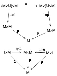
$\mu$ is an arrow from $M\times M \rightarrow M$ , which we’ll call a multiplication operator.
$\eta$ is an arrow from $I \rightarrow M$ , called unit.
$\alpha$ is an arrow from $(M\times M)\times M \rightarrow M \times (M\times M)$ which represents the associativity property of the monoid.
$\lambda$ is a morphism which represents the left identity property of the monoid (that is, $1*x=x$ ), and $\rho$ is a morphism representing the right identity property $(x*1=x)$ .

This diagram, using these arrows, is a way of representing all of the key properties of a monoid via nothing but arrows and composition. It says, among other things, that:

$(M \times M) \times M$ composes with multiplication to be $M \times M$ .
That is, applying multiplication to $(M \times M) \times M$ evaluates to (M \times M).
$(M \times M) \times M$ composed with associativity can become $M \times (M \times M)$ .

So it’s a monoid – but it’s a higher level monoid. In this, $M$ isn’t just an object in a category: it’s an entire category. These arrows are arrows between categories in a category of categories.

What we’ll see when we get deeper into category theory is how powerful this kind of abstraction can get. We’ll often see a sequence of abstractions, where we start with a simple concept (like monoid), and find a way to express it in terms of arrows between objects in a category. But then, we’ll lift it up, and look at how we can see in not just as a relation between objects in a category, but as a different kind of relation between categories, by constructing the same thing using a category of categories. And then we’ll abstract even further, and construct the same thing using mappings between categories of categories.

(You can find the next lesson <a href=”http://www.goodmath.org/blog/2019/02/20/category-theory-lesson-2-basics-of-categorical-abstraction/”>here</a>.)

Monads and Programming

11 Replies

Sorry things have been so slow around here. I know I keep promising that I’m going to post more frequently, but it’s hard. Life as an engineer at a startup is exhausting. There’s so much work to do! And the work is so fun – it’s easy to let it eat up all of your time.

Anyway… last good-math post ’round these parts was about monoids and programming. Today, I’m going to talk about monads and programming!

If you recall, monoids are an algebraic/categorical construct that, when implemented in a programming language, captures the abstract notion of foldability. For example, if you’ve got a list of numbers, you can fold that list down to a single number using addition. Folding collections of values is something that comes up in a lot of programming problems – capturing that concept with a programming construct allows you to write code that exploits the general concept of foldability in many different contexts.

Monads are a construct that have become incredibly important in functional programming, and they’re very, very poorly understood by most people. That’s a shame, because the real concept is actually simple: a monad is all about the concept of sequencing. A monad is, basically, a container that you can wrap something in. Once it’s wrapped, you can form a sequence of transformations on it. The result of each step is the input to the next. That’s really what it’s all about. And when you express it that way, you can begin to see why it’s such an important concept.

I think that people are confused by monads for two reasons:

Monads are almost always described in very, very abstract terms. I’ll also get into the abstract details, but I’ll start by elaborating on the simple description I gave above.
Monads in Haskell, which are where most people are introduced to them, are very confusing. The basic monad operations are swamped with tons of funny symbols, and the basic monad operations are named in incredibly misleading ways. (“return” does almost the exact opposite of what you expect return to do!)

In programming terms, what’s a monad?

Basically, a monadic computation consists of three pieces:

A monadic type, M which is a parametric type wrapper that can wrap a value of any type.
An operation which can wrap a value in M.
An operation which takes a function that transforms a value wraped in M into another value (possibly with a different type) wrapped in M.

Whenever you describe something very abstractly like this, it can seem rather esoteric. But this is just a slightly more formal way of saying what I said up above: it’s a wrapper for a series of transformations on the wrapped value.

Let me give you an example. At foursquare, we do all of our server programming in Scala. In a year at foursquare, I’ve seen exactly one null pointer exception. That’s amazing – NPEs are ridiculously common in Java programming. But in Scala at foursquare, we don’t allow nulls to be used at all. If you have a value which could either be an instance of A, or no value, we use an option type. An Option[T] can be either Some(t: T) or None.

So far, this is nice, but not really that different from a null. The main difference is that it allows you to say, in the type system, whether or not a given value might be null. But: Option is a monad. In Scala, that means that I can use map on it. (map is one of the transformation functions!)

	val t: Option[Int] = ...
	val u: Option[String] = t.map( _ + 2 ).map(_.toString)

What this does is: if t is Some(x), then it adds two to it, and returns Some(x+2); then it takes the result of the first map, and converts it toa string, returning an Option[String]. If t is None, then running map on it always returns None. So I can write code which takes care of the null case, without having to write out any conditional tests of nullness – because optionality is a monad.

In a good implementation of a monad, I can do a bit more than that. If I’ve got a Monad[T], I can use a map-like operation with a function that takes a T and returns a Monad[T].

For an example, we can look at lists – because List is a monad:

val l: List[Int] = List(1, 2, 3)
l.flatMap({ e => List( (e, e), (e+1, e+2) )  })
res0: List[(Int, Int)] = List((1,1), (2,3), (2,2), (3,4), (3,3), (4,5))

The monad map operation does a flatten on the map steps. That means a lot of things. You can see one in the rather silly example above.

You can take values, and wrap them as a list. THen you can perform a series of operations on those elements of a list – sequencing over the elements of the list. Each operation, in turn, returns a list; the result of the monadic computation is a single list, concatenating, in order, the lists returned by each element. In Scala, the flatMap operation captures the monadic concept: basically, if you can flatmap something, it’s a monad.

Let’s look at it a bit more specifically.

The monadic type: List[T].
A function to wrap a value into the monad: the constructor function from List def apply[T](value: T): List[T]
The map operation: def flatMap[T, U](op: T => List[U]): List[U].

(In the original version of this post, the I put the wrong type in flatMap in the list above. In the explanation demonstrating flatMap, the type is correct. Thanks to John Armstrong for catching that!)

You can build monads around just about any kind of type wrapper where it makes sense to map over the values that it wraps: collections, like lists, maps, and options. Various kinds of state – variable environments (where the wrapped values are, essentially, functions from identifiers to values), or IO state. And plenty of other things. Anything where you perform a sequence of operations over a wrapped value, it’s a monad.

Now that we have some understanding of what this thing we’re talking about it, what is it in mathematical terms? For that, we turn to category theory.

Fundamentally, in category theory a monad is a category with a particular kind of structure. It’s a category with one object. That category has a collection of arrows which (obviously) are from the single object to itself. That one-object category has a functor from the category to itself. (As a reminder, a functor is an arrow between categories in the category of (small) categories.)

The first trick to the monad, in terms of theory, is that it’s fundamentally about the functor: since the functor maps from a category to the same category, so you can almost ignore the category; it’s implicit in the definition of the functor. So we can almost treat the monad as if it were just the functor – that is, a kind of transition function.

The other big trick is closely related to that. For the programming language application of monads, we can think of the single object in the category as the set of all possible states. So we have a category object, which is essentially the collection of all possible states; and there are arrows between the states representing possible state transitions. So the monad’s functor is really just a mapping from arrows to different arrows – which basically represents the way that changing the state causes a change in the possible transitions to other states.

So what a monad gives us, in terms of category theory, in a conceptual framework that captures the concept of a state transition system, in terms of transition functions that invisibly carry a state. When that’s translated into programming languages, that becomes a value that implicitly takes an input state, possibly updates it, and returns an output state. Sound familiar?

Let’s take a moment and get formal. As usual for category theory, first there are some preliminary definitions.

Given a category, C, 1_C is the identity functor from C to C.
Given a category C with a functor T : C → C, T² = T º T.
Given a functor T, 1_T : T → T is the natural transformation from T to T.

Now, with that out of the way, we can give the complete formal definition of a monad. Given a category C, a monad on C is a triple: (T:C→C, η:1_C→T, μ:T² → T), where T is a functor, and η and μ are natural transformations. The members of the triple must make the following two diagrams commute.

Commutativity of composition with μ

Commutativity of composition with η

What these two diagrams mean is that successive applications of the state-transition functor over C behave associatively – that any sequence of composing monadic functors will result in a functor with full monadic structure; and that the monadic structure will always preserve. Together, these mean that any sequence of operations (that is, applications of the monad functor) are themselves monad functors – so the building a sequence of monadic state transformers is guaranteed to behave as a proper monadic state transition – so what happens inside of the monadic functor is fine – to the rest of the universe, the difference between a sequence and a single simple operation is indistinguishable: the state will be consistently passed from application to application with the correct chaining behavior, and to the outside world, the entire monadic chain looks like like a single atomic monadic operation.

Now, what does this mean in terms of programming? Each element of a monadic sequence in Haskell is an instantiation of the monadic functor – that is, it’s an arrow between states – a function, not a simple value – which is the basic trick to monads. They look like a sequence of statements; in fact, each statement in a monad is actually a function from state to state. And it looks like we’re writing sequence code – when what we’re actually doing is writing function compositions – so that when we’re done writing a monadic sequence, what we’ve actually done is written a function definition in terms of a sequence of function compositions.

Understanding that, we can now clearly understand why we need the return function to use a non-monad expression inside of a monadic sequence – because each step in the sequence needs to be an instance of the monadic functor; an expression that isn’t an instance of the monadic functor couldn’t be composed with the functions in the sequence. The return function is really nothing but a function that combines a non-monadic expression with the id functor.

In light of this, let’s go back and look at the definition of Monad in the Haskell standard prelude.

class  Functor f  where
  fmap              :: (a -> b) -> f a -> f b

class  Monad m  where
  (>>=)  :: m a -> (a -> m b) -> m b
  (>>)   :: m a -> m b -> m b
  return :: a -> m a
  fail   :: String -> m a

  -- Minimal complete definition:
  --      (>>=), return
  m >> k  =  m >>= _ -> k
  fail s  = error s

The declaration of monad is connected with the definition of functor – if you look, you can see the connection. The fundamental operation of Monad is “>>=” – the chaining operation, which is basically the haskell version of the map operation, which is type m a -> (a -> m b) -> m b is deeply connected with the fmap operation from Functor‘s fmap operation – the a in m a is generally going to be a type which can be a Functor. (Remember what I said about haskell and monads? I really prefer map and flatMap to >> and >>=).

So the value type wrapped in the monad is a functor – in fact, the functor from the category definition! And the “>>=” operation is just the functor composition operation from the monad definition.

A proper implementation of a monad needs to follow some fundamental rules – the rules are, basically, just Haskell translations of the structure-preserving rules about functors and natural transformations in the category-theoretic monad. There are two groups of laws – laws about the Functor class, which should hold for the transition function wrapped in the monad class; and laws about the monadic operations in the Monad class. One important thing to realize about the functor and monad laws is that they are not enforced – in fact, cannot be enforced! – but monad-based code using monad implementations that do not follow them may not work correctly. (A compile-time method for correctly verifying the enforcement of these rules can be shown to be equivalent to the halting problem.)

There are two simple laws for Functor, and it’s pretty obvious why they’re fundamentally just strucure-preservation requirements. The functor class only has one operation, called fmap, and the two functor laws are about how it must behave.

fmap id = id
(Mapping ID over any structured sequence results in an unmodified sequence)
fmap (f . g) = (fmap f) . (fmap g)
(“.” is the function composition operation; this just says that fmap preserves the structure to ensure that that mapping is associative with composition.)

The monad laws are a bit harder, but not much. The mainly govern how monadic operations interact with non-monadic operations in terms of the “return” and “>>=” operations of the Monad class.

return x >>= f = f x
(injecting a value into the monad is basically the same as passing it as a parameter down the chain – return is really just the identity functor passing its result on to the next step. I hate the use of “return”. In a state functor, in exactly the right context, it does sort-of look like a return statement in an imperative language. But in pretty much all real code, return is the function that wraps a value into the monad.)
f >>= return = f
(If you don’t specify a value for a return, it’s the same as just returning the result of the previous step in the sequence – again, return is just identity, so passing something into return shouldn’t affect it.)
seq >>= return . f = fmap f seq
(composing return with a function is equivalent to invoking that function on the result of the monad sequence to that point, and wrapping the result in the monad – in other words, it’s just composition with identity.)
seq >>= (x -> f x >>= g) = (seq >>= f) >>= g
(Your implementation of “>>=” needs to be semantically equivalent to the usual translation; that is, it must behave like a functor composition.)

Introducing Algebraic Data Structures via Category Theory: Monoids

10 Replies

Since joining foursquare, I’ve been spending almost all of my time writing functional programs. At foursquare, we do all of our server programming in Scala, and we have a very strong bias towards writing our scala code very functionally.

This has increased my interest in category theory in an interesting way. As a programming language geek, I’m obviously fascinated by data structures. Category theory provides a really interesting handle on a way of looking at a kind of generic data structures.

Historically (as much as that word can be used for anything in computer science), we’ve thought about data structures primarily in a algorithmic and structural ways.

For example, binary trees. A binary tree consists of a collection of linked nodes. We can define the structure recursively really easily: a binary tree is a node, which contains pointers to at most two other binary trees.

In the functional programming world, people have started to think about things in algebraic ways. So instead of just defining data structures in terms of structure, we also think about them in very algebraic ways. That is, we think about structures in terms of how they behave, instead of how they’re built.

For example, there’s a structure called a monoid. A monoid is a very simple idea: it’s an algebraic structure with a set of values S, one binary operation *, and one value i in S which is an identity value for *. To be a monoid, these objects must satisfy some rules called the monad laws:

$\forall s \in S: s * i = s, i * s = s$
$\forall x, y, z \in S: (x * y) * z = x * (y * z)$

There are some really obvious examples of monoids – like the set of integers with addition and 0 or integers with multiplication and 1. But there are many, many others.

Lists with concatenation and the empty list are a monoid: for any list,
l ++ [] == l, [] + l == l, and concatenation is associative.

Why should we care if data structures like are monoids? Because we can write very general code in terms of the algebraic construction, and then use it over all of the different operations. Monoids provide the tools you need to build fold operations. Every kind of fold – that is, operations that collapse a sequence of other operations into a single value – can be defined in terms of monoids. So you can write a fold operation that works on lists, strings, numbers, optional values, maps, and god-only-knows what else. Any data structure which is a monoid is a data structure with a meaningful fold operation: monoids encapsulate the requirements of foldability.

And that’s where category theory comes in. Category theory provides a generic method for talking about algebraic structures like monoids. After all, what category theory does is provide a way of describing structures in terms of how their operations can be composed: that’s exactly what you want for talking about algebraic data structures.

The categorical construction of a monoid is, alas, pretty complicated. It’s a simple idea – but defining it solely in terms of the composition behavior of function-like objects does take a bit of effort. But it’s really worth it: when you see a monoidal category, it’s obvious what the elements are in terms of programming. And when we get to even more complicated structures, like monads, pullbacks, etc., the advantage will be even clearer.

A monoidal category is a category with a functor, where the functor has the basic properties of a algebraic monoid. So it’s a category C, paired with a bi-functor – that is a two-argument functor ⊗:C×C→C. This is the categorical form of the tensor operation from the algebraic monoid. To make it a monoidal category, we need to take the tensor operation, and define the properties that it needs to have. They’re called its coherence conditions, and basically, they’re the properties that are needed to make the diagrams that we’re going to use commute.

So – the tensor functor is a bifunctor from C×C to C. There is also an object I∈C, which is called the unit object, which is basically the identity element of the monoid. As we would expect from the algebraic definition, the tensor functor has two basic properties: associativity, and identity.

Associativity is expressed categorically using a natural isomorphism, which we’ll name α. For any three object X, Y, and Z, α includes a component α_X,Y,Z (which I’ll label α(X,Y,Z) in diagrams, because subscripts in diagrams are a pain!), which is a mapping from (X⊗Y)⊗Z to X⊗(Y⊗Z). The natural isomorphism says, in categorical terms, that the the two objects on either side of its mappings are equivalent.

The identity property is again expressed via natural isomorphism. The category must include an object I (called the unit), and two natural isomorphisms, called &lamba; and ρ. For any arrow X in C, &lamba; and ρ contain components λ_X and ρ_X such that λ_X maps from I⊗X→X, and ρ_X maps from X⊗I to X.

Now, all of the pieces that we need are on the table. All we need to do is explain how they all fit together – what kinds of properties these pieces need to have for this to – that is, for these definitions to give us a structure that looks like the algebraic notion of monoidal structures, but built in category theory. The properties are, more or less, exact correspondences with the associativity and identity requirements of the algebraic monoid. But with category theory, we can say it visually. The two diagrams below each describe one of the two properties.

The upper (pentagonal) diagram must commute for all A, B, C, and D. It describes the associativity property. Each arrow in the diagram is a component of the natural isomorphism over the category, and the diagram describes what it means for the natural isomorphism to define associativity.

Similarly, the bottom diagram defines identity. The arrows are all components of natural isomorphisms, and they describe the properties that the natural isomorphisms must have in order for them, together with the unit I to define identity.

Like I said, the definition is a lot more complicated. But look at the diagram: you can see folding in it, in the chains of arrows in the commutative diagram.

Categorical Equalizers

Substuff

2 Replies

What’s a subset? That’s easy: if we have two sets A and B, A is a subset of B if every member of A is also a member of B.

We can take the same basic idea, and apply it to something which a tad more structure, to get subgroups. What’s a subgroup? If we have two groups A and B, and the values in group A are a subset of the values in group B, then A is a subgroup of B.

The point of category theory is to take concepts like “subset” and generalize them so that we can apply the same idea in many different domains. In category theory, we don’t ask “what’s a subset?”. We ask, for any structured THING, what does it mean to be a sub-THING? We’re being very general here, and that’s always a bit tricky. We’ll start by building a basic construction, and look at it in terms of sets and subsets, where we already understand the specific concept.

In terms of sets, the most generic way of defining subsets is using functions. Suppose we have a set, A. How can we define all of the subsets of A, in terms of functions? We can do it using injective functions, as follows. (As a reminder, a function from X to Y where every value in X is mapped to a distinct function in y.)

For the set, A, we can take the set of all injective functions to A. We’ll call that set of functions Inj(A).

Given Inj(A), we can define equivalence classes over Inj(A), so that $f: X \rightarrow A$ and $g: Y \rightarrow A$ are equivalent if there is an isomorphism between X and Y.

The domain of each function in one of the equivalence classes in Inj(A) is a function isomorphic to a subset of A. So each equivalence class of injective functions defines a subset of A.

And there we go: we’ve got a very abstract definition of subsets.

Now we can take that, and generalize that function-based definition to categories, so that it can define a sub-object of any kind of object that can be represented in a category.

Before we jump in, let me review one important definition from before; the monomorphism, or monic arrow.

A monic arrow is an arrow $f : a \rightarrow b$ such that
$\forall g_1, g_2: x \rightarrow a: f \circ g_1 \ge f \circ g_2 \Rightarrow g_1 = g_2$ (That is, if any two arrows composed with $f$ in $f \circ g$ end up at the same object only if they are the same.)

So, basically, the monic arrow is the category theoretic version of an injective function. We’ve taken the idea of what an injective function means, in terms of how functions compose, and when we generalized it, the result is the monic arrow.

Suppose we have a category $C$ , and an object $a in \mbox{Obj}(C)$ . If there are are two monic arrows $f : x \rightarrow a$ and $g : y \rightarrow a$ , and
there is an arrow $h$ such that $g \circ h = f$ , then we say $f \le g$ (read “f factors through g”). Now, we can take that “≤” relation, and use it to define an equivalence class of morphisms using $f \equiv g \Leftrightarrow f \le g \land g \le f$ .

What we wind up with using that equivalence relation is a set of equivalence classes of monomorphisms pointing at A. Each of those equivalence classes of morphisms defines a subobject of A. (Within the equivalence classes are objects which have isomorphisms, so the sources of those arrows are equivalent with respect to this relation.) A subobject of A is the sources of an arrow in one of those equivalence classes.

It’s exactly the same thing as the function-based definition of sets. We’ve created a very general concept of sub-THING, which works exactly the same way as sub-sets, but can be applied to any category-theoretic structure.

Interpreting Lambda Calculus using Closed Cartesian Categories

3 Replies

Today I’m going to show you the basic idea behind the equivalency of closed cartesian categories and typed lambda calculus. I’ll do that by showing you how the λ-theory of any simply typed lambda calculus can be mapped onto a CCC.

First, let’s define the term “lambda theory”. In the simply typed lambda calculus, we always have a set of base types – the types of simple atomic values that can appear in lambda expressions. A lambda theory is a simply typed lambda calculus, plus a set of additional rules that define equivalences over the base types.

So, for example, if one of the base types of a lambda calculus was the natural numbers, the lambda theory would need to include rules to define equality over the natural numbers:

x = y if x=0 and y=0; and
x = y if x=s(x’) and y=s(y’) and x’ = y’

So. Suppose we have a lambda-theory $L$ . We can construct a corresponding category $C(L)$ . The objects in $C(L)$ are the types in $L$ . The arrows in $C(L)$ correspond to families of expressions in $L$ ; an arrow
$f : A \rightarrow B$ corresponds to the set of expressions of type $B$ that contain a single free variable of type $A$ .

The semantics of the lambda-theory can be defined by a functor; in particular, a cartesian closed functor $F$ that maps from $C(L)$ to the closed cartesian category of Sets. (It’s worth noting that this is completely equivalent to the normal Kripke semantics for lambda calculus; but when you get into more complex lambda calculi, like Hindley-Milner variants, this categorical formulation is much simpler.)

We describe how we build the category for the lambda theory in terms of a CCC using something called an interpretation function. It’s really just a notation that allows us to describe the translation recursively. The interpretation function is written using brackets: $[A]$ is the categorical interpretation of the type $A$ from lambda calculus.

So, first, we define an object for each type in $L$ . We need to include a special
type, which we call unit. The idea behind unit is that we need to be able to talk about “functions” that either don’t take any real paramaters, or functions that don’t return anything. Unit is a type which contains exactly one atomic value. Since there’s only one possible value for unit, and unit doesn’t have any extractable sub-values, conceptually, it doesn’t ever need to be passed around. So it’s a “value” that never needs to get passed – perfect for a content-free placeholder.

Anyway, here we go with the base rules:

$\forall A \in \mbox{basetypes}(L), [A] = A_C \in C(L)$
$[\mbox{unit}] = 1_C$

Next, we need to define the typing rules for complex types:

$[ A \times B] == [A] \times [B]$
$[A \rightarrow B] = [B]^{[A]}$

Now for the really interesting part. We need to look at type derivations – that is, the type inference rules of the lambda calculus – to show how to do the correspondences between more complicated expressions. Just like we did in lambda calculus, the type derivations are done with a context $Gamma$ , containing a set of type judgements. Each type judgement assigns a type to a lambda term. There are two translation rules for contexts:

$[ \emptyset ] = 1_C$
$[\Gamma, x: A] = [\Gamma] \times [A]$

We also need to describe what to do with the values of the primitive types:

For each value $v : A$ , there is an arrow $v : 1 \rightarrow A_C$ .

And now the rest of the rules. Each of these is of the form $[\Gamma :- x : A] = \mbox{arrow}$ , where we’re saying that $\Gamma$ entails the type judgement $x : A$ . What it means is the object corresponding to the type information covering a type inference for an expression corresponds to the arrow in $C(L)$ .

Unit evaluation: $[ \Gamma :- \mbox{unit}: \mbox{Unit}] = !: [\Gamma] \rightarrow [\mbox{Unit}]$ . (A unit expression is a special arrow “!” to the unit object.)
Simple Typed Expressions: $[\Gamma :- a: A_C] = a \circ ! : [\Gamma] \rightarrow [A_C]$ . (A simple value expression is an arrow composing with ! to form an arrow from Γ to the type object of Cs type.)
Free Variables: $[\Gamma x: A :- x : A] = \pi_2 : ([\Gamma] \times [A]) \rightarrow [A]$ (A term which is a free variable of type A is an arrow from the product of Γ and the type object A to A; That is, an unknown value of type A is some arrow whose start point will be inferred by the continued interpretation of gamma, and which ends at A. So this is going to be an arrow from either unit or a parameter type to A – which is a statement that this expression evaluates to a value of type A.)
Inferred typed expressions: $[\Gamma, x:A :- x$ , where $\pi_1: ([\Gamma] \times [A])\rightarrow [A']$ (If the type rules of Γ plus the judgement $x : A$ gives us $x$ , then the term $x$ is an arrow starting from the product of the interpretation of the full type context with $A$ ), and ending at $A'$ . This is almost the same as the previous rule: it says that this will evaluate to an arrow for an expression that results in type $A$ .)
Function Abstraction: $[\Gamma :- \lambda x:A . M : A \rightarrow B] = \mbox{curry}([\Gamma, x:A :- M:B]) : [\Gamma] \rightarrow B^{[A]}$ . (A function maps to an arrow from the type context to an exponential $[B]^{[A]}$ , which is a function from $A$ to $B$ .)
Function application: $[\Gamma :- (M M'): B] = \mbox{eval}_{C, B} \circ ([\Gamma :- M: C \rightarrow B]$ , $[\Gamma :- (M M'): B] = \mbox{eval}_{C,B} \circ ([\Gamma :- M : C \rightarrow B]$ , $[\Gamma :- M': C]): [\Gamma] \rightarrow [B]$ . (function evaluation takes the eval arrow from the categorical exponent, and uses it to evaluate out the function.)

There are also two projection rules for the decomposing categorical products, but they’re basically more of the same, and this is already dense enough.

The intuition behind this is:

arrows between types are families of values. A particular value is a particular arrow from unit to a type object.
the categorical exponent in a CC is exactly the same thing as a function type in λ-calculus; and an arrow to an exponent is the same thing as a function value. Evaluating the function is using the categorical exponent’s eval arrow to “decompose” the exponent, and produce an arrow to the function’s result type; that arrow is the value that the function evaluates to.
And the semantics – called functorial semantics – maps from the objects in this category, $C(L)$ to the category of Sets; function values to function arrows; type objects to sets; values to value objects and arrows. (For example, the natural number type would be an object in $C(L)$ , and the set of natural numbers in the sets category would be the target of the functor.)

Aside from the fact that this is actually a very clean way of defining the semantics of a not-so-simply typed lambda calculus, it’s also very useful in practice. There is a way of executing lambda calculus expressions as programs that is based on this, called the Categorical Abstract Machine. The best performing lambda-calculus based programming language (and my personal all-time-favorite programming language), Objective-CAML had its first implementation based on the CAM. (CAML stands for categorical abstract machine language.).

From this, you can see how the CCCs and λ-calculus are related. It turns out that that relation is not just cool, but downright useful. Concepts from category theory – like monads, pullbacks, and functors are really useful things in programming languages! In some later posts, I’ll talk a bit about that. My current favorite programming language, Scala, is one of the languages where there’s a very active stream of work in applying categorical ideas to real-world programming problems.

Sidetrack from the CCCs: Lambda Calculus

3 Replies

So, last post, I finally defined closed cartesian categories. And I alluded to the fact that the CCCs are, essentially, equivalent to the simply typed λ calculus. But I didn’t really talk about what that meant.

Before I can get to that, you need to know what λ calculus is. Many readers are probably familiar, but others aren’t. And as it happens, I absolutely love λ calculus.

In computer science, especially in the field of programming languages, we tend to use λ calculus a whole lot. It’s also extensively used by logicians studying the nature of computation and the structure of discrete mathematics. λ calculus is great for a lot of reasons, among them:

It’s very simple.
It’s Turing complete: if a function can be computed by any possible computing device, then it can be written in λ-calculus.
It’s easy to read and write.
Its semantics are strong enough that we can do reasoning from it.
It’s got a good solid model.
It’s easy to create variants to explore the properties of various alternative ways of structuring computations or semantics.

The ease of reading and writing λ calculus is a big deal. It’s led to the development of a lot of extremely good programming languages based, to one degree or another, on the λ calculus: Lisp, ML, Haskell, and my current favorite, Scala, are very strongly λ calculus based.

The λ calculus is based on the concept of functions. In the pure λ calculus, everything is a function; there are no values except for functions. In fact, we can pretty much build up all of mathematics using λ-calculus.

With the lead-in out of the way, let’s dive in a look at λ-calculus. To define a calculus, you need to define two things: the syntax, which describes how valid expressions can be written in the calculus; and a set of rules that allow you to symbolically manipulate the expressions.

Lambda Calculus Syntax

The λ calculus has exactly three kinds of expressions:

Function definition: a function in λ calculus is an expression, written: λ param . body, which defines a function with one parameter.
Identifier reference: an identifier reference is a name which matches the name of a parameter defined in a function expression enclosing the reference.
Function application: applying a function is written by putting the function value in front of its parameter, as in x y to apply the function x to the value y.

There’s a trick that we play in λ calculus: if you look at the definition above, you’ll notice that a function (lambda expression) only takes one parameter. That seems like a very big constraint – how can you even implement addition with only one parameter?

It turns out to be no problem, because of the fact that functions are, themselves, values. Instead of writing a two parameter function, you can write a one parameter function that returns a one parameter function, which can then operate on the second parameter. In the end, it’s effectively the same thing as a two parameter function. Taking a two-parameter function, and representing it by two one-parameter functions is called currying, after the great logician Haskell Curry.

For example, suppose we wanted to write a function to add x and y. We’d like to write something like: λ x y . x + y. The way we do that with one-parameter functions is: we first write a function with one parameter, which returns another function with one parameter.

Adding x plus y becomes writing a one-parameter function with parameter x, which returns another one parameter function which adds x to its parameter: λ x . (λ y . x + y).

Now that we know that adding multiple parameter functions doesn’t really add anything but a bit of simplified syntax, we’ll go ahead and use them when it’s convenient.

One important syntactic issue that I haven’t mentioned yet is closure or complete binding. For a λ calculus expression to be evaluated, it cannot reference any identifiers that are not bound. An identifier is bound if it a parameter in an enclosing λ expression; if an identifier is not bound in any enclosing context, then it is called a free variable. Let’s look quickly at a few examples:

λ x . p x y: in this expression, y and p are free, because they’re not the parameter of any enclosing λ expression; x is bound because it’s a parameter of the function definition enclosing the expression p x y where it’s referenced.
λ x y.y x: in this expression both x and y are bound, because they are parameters of the function definition, and there are no free variables.
λ y . (λ x . p x y). This one is a tad more complicated, because we’ve got the inner λ. So let’s start there. In the inner λ, λ x . p x y, y and p are free and x is bound. In the full expression, both x and y are bound: x is bound by the inner λ, and y is bound by the other λ. “p” is still free.

We’ll often use “free(x)” to mean the set of identifiers that are free in the expression “x”.

A λ calculus expression is valid (and thus evaluatable) only when all of its variables are bound. But when we look at smaller subexpressions of a complex expression, taken out of context, they can have free variables – and making sure that the variables that are free in subexpressions are treated right is very important.

Lambda Calculus Evaluation Rules

There are only two real rules for evaluating expressions in λ calculus; they’re called α and β. α is also called “conversion”, and β is also called “reduction”.

α is a renaming operation; basically it says that the names of variables are unimportant: given any expression in λ calculus, we can change the name of the parameter to a function as long as we change all free references to it inside the body.

So – for instance, if we had an expression like:

λ x . if (= x 0) then 1 else x^2

We can do an α to replace X with Y (written “α[x/y]” and get):

λ y . if (= y 0) then 1 else y^2

Doing α does not change the meaning of the expression in any way. But as we’ll see later, it’s important because without it, we’d often wind up with situations where a single variable symbol is bound by two different enclosing λs. This will be particularly important when we get to recursion.

β reduction is where things get interesting: this single rule is all that’s needed to make the λ calculus capable of performing any computation that can be done by a machine.

β basically says that if you have a function application, you can replace it with a copy of the body of the function with references to the parameter identifiers replaced by references to the parameter value in the application. That sounds confusing, but it’s actually pretty easy when you see it in action.

Suppose we have the application expression: (λ x . x + 1) 3. By performing a beta reduction, we can replace the application by taking the body x + 1 of the function, and substituting (or αing) the value of the parameter (3) for the parameter variable symbol (x). So we replace all references to x with 3. So the result of doing a beta reduction xs 3 + 1.

A slightly more complicated example is the expression:

λ y . (λ x . x + y)) q

It’s an interesting expression, because it’s a λ expression that when applied, results in another λ expression: that is, it’s a function that creates functions. When we do beta reduction in this, we’re replacing all references to the parameter y with the identifier q; so, the result is λ x . x + q.

One more example, just for the sake of being annoying. Suppose we have: (λ x y. x y) (λ z . z * z) 3

That’s a function that takes two parameters, and applies the first one to the second one. When we evaluate that, we replace the parameter x in the body of the first function with λ z . z * z; and we replace the parameter y with 3, getting: (λ z . z * z) 3. And we can perform beta on that, getting 3 * 3.

Written formally, beta says: λ x . B e = B[x := e] if free(e) ⊂ free(B[x := e])

That condition on the end, “if free(e) ⊂ free(B[x := e]” is why we need α: we can only do beta reduction if doing it doesn’t create any collisions between bound identifiers and free identifiers: if the identifier “z” is free in “e”, then we need to be sure that the beta-reduction doesn’t make “z” become bound. If there is a name collision between a variable that is bound in “B” and a variable that is free in “e”, then we need to use α to change the identifier names so that they’re different.

As usual, an example will make that clearer: Suppose we have a expression defining a function, λ z . (λ x . x+z). Now, suppose we want to apply it: (λ z . (λ x . x + z)) (x + 2). In the parameter (x + 2), x is free. Now, suppose we break the rule and go ahead and do beta. We’d get “λ x . x + x + 2“. The variable that was free in x + 2 is now bound! We’ve changed the meaning of the function, which we shouldn’t be able to do. If we were to apply that function after the incorrect β, we’d get (λ x . x + x + 2) 3. By beta, we’d get 3 + 3 + 2, or 8.

What if we did α the way we were supposed to?

First, we’d do an α to prevent the name overlap. By α[x/y], we would get λ z . (λ y . y + z) (x+2).

Then by β, we’d get “λ y . y + x + 2“. If we apply this function the way we did above, then by β, we’d get 3+x+2.
3+x+2 and 3+3+2 are very different results!

And that’s pretty much it. There’s another optional rule you can add called η-conversion. η is a rule that adds extensionality, which provides a way of expressing equality between functions.

η says that in any λ expression, I can replace the value f with the value g if/f for all possible parameter values x, f x = g x.

What I’ve described here is Turing complete – a full effective computation system. To make it useful, and see how this can be used to do real stuff, we need to define a bunch of basic functions that allow us to do math, condition tests, recursion, etc. I’ll talk about those in my next post.

It’l also important to point out that while I’ve gone through a basic definition of λ calculus, and described its mechanics, I haven’t yet defined a model for λ-calculus. That’s quite an important omission! λ-calculus was played with by logicians for several years before they were able to come up with a complete model for it, and it was a matter of great concern that although it looked correct, the early attempts to define a model for it were failures! And without a valid model, the results of the system are meaningless. An invalid model in a logical system like calculus is like a contradiction in axioms: it means that nothing that it produces is valid.

Categorical Computation Characterized By Closed Cartesian Categories

3 Replies

One of my favorite categorical structures is a thing called a closed cartesian category, or CCC for short. Since I’m a computer scientist/software engineer, it’s a natural: CCCs are, basically, the categorical structure of lambda calculus – and thus, effectively, a categorical model of computation. However, before we can talk about the CCCs, we need – what else? – more definitions.

Cartesian Categories

A cartesian category $C$ (note not cartesian closed category) is a category:

With a terminal object $t$ , and
$forall a, b in Obj(C)$ , the objects and arrows of the categorical product $a times b in C$ .

So, a cartesian category is a category closed with respect to product. Many of the common categories are cartesian: the category of sets, and the category of enumerable sets, And of course, the meaning of the categorical product in set? Cartesian product of sets.

Categorical Exponentials

To get from cartesian categories to cartesian closed categories, we also need to define categorical exponentials. Like categorical product, the value of a categorical exponential is not required to included in a category. The exponential is a complicated definition, and it’s a bit hard to really get your head around, but it’s well worth the effort. If categorical products are the categorical generalization of set products, then the categorical exponential is the categorical version of a function space. It gives us the ability to talk about structures that are the generalized version of “all functions from A to B”.

Given two objects x and y from a category C, their categorical exponential x^y, if it exists in the category, is defined by a set of values:

An object $x^y$ ,
An arrow $mbox{eval}_{y,x}: x^y times y rightarrow x$ , called an evaluation map.
$forall z in Obj(C)$ , an operation $Lambda_C: (z times y rightarrow x) rightarrow (z rightarrow x^y)$ . (That is, an operation mapping from arrows to arrows.)

These values must have the following properties:

:
- $mbox{val}_{y,x} circ (Lambda_C(f)times 1_y)$
- $forall f : z times y rightarrow x, g : z rightarrow x^y: Lambda_C(mbox{eval}_{y,x} circ (z times 1_y) = z$

To make that a bit easier to understand, let’s turn it into a diagram.

As I alluded to earlier, you can also think of it as a generalization of a function space. $x^y$ is the set of all functions from y to x. The evaluation map is simple description in categorical terms of an operation that applies a function from a to b (an arrow) to a value from a, resulting in an a value from b.

So what does the categorical exponential mean? I think it’s easiest to explain in terms of sets and functions first, and then just step it back to the more general case of objects and arrows.

If X and Y are sets, then $X^Y$ is the set of functions from Y to X.

Now, look at the diagram:

The top part says, basically, that $g$ is a function from $Z$ to to $X^Y$ : so $g$ takes a member of $Z$ , and uses it to select a function from $Y$ to $X$ .
The vertical arrow says:
1. given the pair $(z,y)$ , $f(z,y)$ maps $(z,y)$ to a value in $X$ .
2. given a pair , we’re going through a function. It’s almost like currying:
  1. The vertical arrow going down is basically taking $g(z,y)$ , and currying it to $g(z)(y)$ .
  2. Per the top part of the diagram, $g(z)$ selects a function from $y$ to $x$ . (That is, a member of $X^Y$ .)
  3. So, at the end of the vertical arrow, we have a pair $(g(z), y)$ .
3. The “eval” arrow maps from the pair of a function and a value to the result of applying the function to the value.
Cartesian Closed Categories

Now – the abstraction step is actually kind of easy: all we’re doing is saying that there is a structure of mappings from object to object here. This particular structure has the essential properties of what it means to apply a function to a value. The internal values and precise meanings of the arrows connecting the values can end up being different things, but no matter what, it will come down to something very much like function application.

With exponentials and products, we can finally say what the cartesian closed categories (CCCs). A Cartesian closed category is a category that is closed with respect to both products and exponentials.

Why do we care? Well, the CCCs are in a pretty deep sense equivalent to the simply typed lambda calculus. That means that the CCCs are deeply tied to the fundamental nature of computation. The structure of the CCCs – with its closure WRT product and exponential – is an expression of the basic capability of an effective computing system. So next, we’ll take a look at a couple of examples of what we can do with the CCCs as a categorical model of computation.
Share this:
Like this:
Like Loading...

Building Structure in Category Theory: Definitions to Build On

3 Replies

The thing that I think is most interesting about category theory is that what it’s really fundamentally about is structure. The abstractions of category theory let you talk about structures in an elegant way; and category diagrams let you illustrate structures in a simple visual way. Morphisms express the structure of a category; functors are higher level morphisms that express the structure of relationships between categories.

In my last category theory post, I showed how you can use category theory to describe the basic idea of symmetry and group actions. Symmetry is, basically, an immunity to transformation – that is, a kind of structural property of an object or system where applying some kind of transformation to that object doesn’t change the object in any detectable way. The beauty of category theory is that it makes that definition much simpler.

Symmetry transformations are just the tip of the iceberg of the kinds of structural things we can talk about using categories. Category theory lets you build up pretty much any mathematical construct that you’d like to study, and describe transformations on it in terms of functors. In fact, you can even look at the underlying conceptual structure of category theory using category theory itself, by creating a category in which categories are objects, and functors are the arrows between categories.

So what happens if we take the same kind of thing that we did to get group actions, and we pull out a level, so that instead of looking at the category of categories, focusing on arrows from the specific category of a group to the category of sets, we do it with arrows between members of the category of functors?

We get the general concept of a natural transformation. A natural transformation is a morphism from functor to functor, which preserves the full structure of morphism composition within the categories mapped by the functors. The original inventor of category theory said that natural transformations were the real point of category theory – they’re what he wanted to study.

Suppose we have two categories, C and D. And suppose we also have two functors, F, G : C → D. A natural transformation from F to G, which we’ll call η maps every object x in C to an arrow η_x : F(x) → G(x). η_x has the property that for every arrow a : x → y in C, η_y º F(a) = G(a) º η_x. If this is true, we call η_x the component of η for (or at) x.

That paragraph is a bit of a whopper to interpret. Fortunately, we can draw a diagram to help illustrate what that means. The following diagram commutes if η has the property described in that paragraph.

I think this is one of the places where the diagrams really help. We’re talking about a relatively straightforward property here, but it’s very confusing to write about in equational form. But given the commutative diagram, you can see that it’s not so hard: the path η_y º F(a) and the path G(a) º η<sub compose to the same thing: that is, the transformation η hasn’t changed the structure expressed by the morphisms.

And that’s precisely the point of the natural transformation: it’s a way of showing the relationships between different descriptions of structures – just the next step up the ladder. The basic morphisms of a category express the structure of the category; functors express the structure of relationships between categories; and natural transformations express the structure of relationships between relationships.

Of course, this being a discussion of category theory, we can’t get any further without some definitions. To get to some of the interesting material that involves things like natural transformations, we need to know about a bunch of standard constructions: initial and final objects, products, exponentials… Then we’ll use those basic constructs to build some really fascinating constructs. That’s where things will get really fun.

So let’s start with initial and finial objects.

An initial object is a pretty simple idea: it’s an object with exactly one arrow to each of the other objects in the category. To be formal, given a category $C$ , an object $o \in Obj(C)$ is an initial object if and only if $\forall b \in Obj(c): \exists_1 f: o \rightarrow b \in Mor(C)$ . We generally write $0_c$ for the initial object in a category. Similarly, there’s a dual concept of a terminal object $1_c$ , which is object for which there’s exactly one arrow from every object in the category to $1_c$ .

Given two objects in a category, if they’re both initial, they must be isomorphic. It’s pretty easy to prove: here’s the sketch. Remember the definition of isomorphism in category theory. An isomorphism is an arrow $f : a \rightarrow b$ , where $\exists g : b \rightarrow a)$ such that $f \circ g = 1_b$ and $g \circ f = 1_a$ . If an object is initial, then there’s an arrow from it to every other object — including the other initial object. And there’s an arrow back, because the other one is initial. The iso-arrows between the two initials obviously compose to identities.

Now, let’s move on to categorical products. Categorical products define the product of two objects in a category. The basic concept is simple – it’s a generalization of cartesian product of two sets. It’s important because products are one of the major ways of building complex structures using simple categories.

Given a category $C$ , and two objects $a,b \in Obj(C)$ , the categorical product $a times b$ consists of:

An object $p$ , often written $a \times b$ ;
two arrows $p_a$ and $p_b$ , where $p \in Obj(C)$ , $p_a : p \rightarrow a$ , and $p_b : p \rightarrow b$ .
a “pairing” operation, which for every object , maps the pair of arrows and
to an arrow , where has the
following properties:
1. $p_a \circ \langle f,g \rangle = f$
2. $p_b \circ \langle f,g \rangle = g$
3. $\forall h : c \rightarrow a \times b: \langle p_a \circ h, p_b \circ h \rangle = h$

The first two of those properties are the separation arrows, to get from the product to its components; and the third is the merging arrow, to get from the components to the product. We can say the same thing about the relationships in the product in an easier way using a commutative diagram:

One important thing to understand is that categorical products do not have to exist. This definition doen not say that given any two objects $a$ and $b$ , that $a times b$ is a member of the category. What it says is what the categorical product
looks like if it exists. If, for a given pair a and b of objects, there is an object that meets this definition, then the product of a and b exists in the category. If not, it doesn’t. For many categories, the products don’t exist for some or even all of the objects in the category. But as we’ll see later, the categories for which the products do exist have some really interesting properties.

Defining Categories

Example: The category Set

Example: The category Poset

Commuting Diagrams

Diagrams and Meta-level reasoning: an example

Categorizing Things

Monics, Epics, and Isos

Initial and Terminal Objects

A brief interlude:

Constructions

Products

Share this:

Like this:

Introduction and Motivation

What’s the point?

Start with an Example: Monoids

Monoids in Code

From Sets to Arrows

Deeper Into Arrows

Share this:

Like this:

Share this:

Like this:

Share this:

Like this:

Share this:

Like this:

Share this:

Like this:

Share this:

Like this:

Lambda Calculus Syntax

Lambda Calculus Evaluation Rules

Share this:

Like this:

Cartesian Categories

Categorical Exponentials

Cartesian Closed Categories

Share this:

Like this:

Share this:

Like this: