Category Archives: Uncategorized

How Computers Work: Arithmetic With Gates

In my last post, I promised that I’d explain how we can build interesting mathematical operations using logic gates. In this post, I’m going to try do that by walking through the design of a circuit that adds to multi-bit integers together.

As I said last time, most of the time, when we’re trying to figure out how to do something with gates, it’s useful to with boolean algebra to figure out what we want to build. If we have two bits, what does it mean, in terms of boolean logic to add them?

Each input can be either 0 or 1. If they’re both one, then the sum is 0. If either, but not both, is one, then the sum is 1. If both are one, then the sum is 2. So there’s three possible outputs: 0, 1, and 2.

This brings us to the first new thing: we’re building something that operates on single bits as inputs, but it needs to have more than one bit of output! A single boolean output can only have two possible values, but we need to have three.

The way that we usually describe it is that a single bit adder takes two inputs, X and Y, and produces two outputs, SUM and CARRY. Sum is called the “low order” bit, and carry is the “high order” bit – meaning that if you interpret the output as a binary number, you put the higher order bits to the left of the low order bits. (Don’t worry, this will get clearer in a moment!)

Let’s look at the truth table for a single bit adder, with a couple of extra columns to help understand how we intepret the outputs:

XYSUMCARRYBinaryDecimal
0000000
0110011
1010011
1101102

If we look at the SUM bit, it’s an XOR – that is, it outputs 1 if exactly one, but not both, of its inputs is 1; otherwise, it outputs 0. And if we look at the carry bit, it’s an AND. Our definition of one-bit addition is thus:

  • SUM = X \oplus Y
  • CARRY = X \land Y

We can easily build that with gates:

A one-bit half-adder

This little thing is called a half-adder. That may seem confusing at first, because it is adding two one-bit values. But we don’t really care about adding single bits. We want to add numbers, which consist of multiple bits, and for adding pairs of bits from multibit numbers, a half-adder only does half the work.

That sounds confusing, so let’s break it down a bit with an example.

  • Imagine that we’ve got two two bit numbers, 1 and 3 that we want to add together.
  • In binary 1 is 01, and 3 is 11.
  • If we used the one-bit half-adders for the 0 bit (that is, the lowest order bit – in computer science, we always start counting with 0), we’d get 1+1=0, with a carry of 1; and for the 1 bit, we’d get 1+0=1 with a carry of 0. So our sum would be 10, which is 2.
  • That’s wrong, because we didn’t do anything with the carry output from bit 0. We need to include that as an input to the sum of bit 1.

We could try starting with the truth table. That’s always a worthwile thing to do. But it gets really complicated really quickly.

XX0X1YY0Y1OUTOUT0CARRY0OUT1CARRY1
00000000000
00011011000
00020120010
00031131010
11000011000
11011020110
11020131010
11031140101
20100020010
20111031010
20120140001
20131151011
31100031010
31111040111
31120151011
31131160111

This is a nice illustration of why designing CPUs is so hard, and why even massively analyzed and tested CPUs still have bugs! We’re looking at one of the simplest operations to implement; and we’re only looking at it for 2 bits of input. But already, it’s hard to decide what to include in the table, and to read the table to understand what’s going on. We’re not really going to be able to do much reasoning here directly in boolean logic using the table. But it’s still good practice, both because it helps us make sure we understand what outputs we want, and because it gives us a model to test against once we’ve build the network of gates.

And there’s still some insight to be gained here: Look at the row for 1 + 3. In two bit binary, that’s 01 + 11. The sum for bit 0 is 0 – there’s no extra input to worry about,
but it does generate a carry out. The sum of the input bits for bit
one is 1+1=10 – so 0 with a carry bit. But we have the carry from bit
0 – that needs to get added to the sum for bit1. If we do that – if we do another add step to add the carry bit from bit 0 to the sum from bit 1, then we’ll get the right result!

The resulting gate network for two-bit addition looks like:

The adder for bit 1, which is called a full adder, adds the input bits X1 and Y1, and then adds the sum of those (produced by that first adder) to the carry bit from bit0. With this gate network, the output from the second adder for bit 1 is the correct value for bit 1 of the sum, but we’ve got two different carry outputs – the carry from the first adder for bit 1, and the carry from the second adder. We need to combine those somehow – and the way to do it is an OR gate.

Why an OR gate? The second adder will only produce a carry if the first adder produced a 1 as its output. But there’s no way that adding two bits can produce both a 1 as its sum output and a 1 as its carry output. So the carry bit from the second adder will only ever be 1 if the output of the first adder is 0; and the carry output from the first adder will only ever be 1 if the sum output from the first carry is 0. Only one of the two carries will ever be true, but if either of them is true, we should produce a 1 as the carry output. Thus, the or-gate.

Our full adder, therefore, takes 3 inputs: a carry from the next lower bit, and the two bits to sum; and it outputs two bits: a sum and a carry. Inside, it’s just two adders chained together, so that first we add the two sum inputs, and then we add the sum of that to the incoming carry.

For more than two bits, we just keep chaining full adders together. For example,
here’s a four-bit adder.

This way of implementing sum is called a ripple carry adder – because the carry bits ripple up through the gates. It’s not the most efficient way of producing a sum – each higher order bit of the inputs can’t be added together until the next lower bit is done, so the carry ripples through the network as each bit finishes, and the total time required is proportional to the number of bits to be summed. More bits means that the ripple-carry adder gets slower. But this works, and it’s pretty easy to understand.

There are faster ways to build multibit adders, by making the gate network more complicated in order to remove the ripple delay. You can imagine, for example, that instead of waiting for the carry from bit 0, you could just build the circuit for bit 1 so that it inputs X0 and Y0; and similarly, for bit 2, you could include X0, X1, Y0, and Y1 as additional inputs. You can imagine how this gets complicated quickly, and there are some timing issues that come up as the network gets more complicated, which I’m really not competent to explain.

Hopefully this post successfully explained a bit of how interesting operations like arithmetic can be implemented in hardware, using addition as an example. There are similar gate networks for subtraction, multiplication, etc.

These kinds of gate networks for specific operations are parts of real CPUs. They’re called functional units. In the simplest design, a CPU has one functional unit for each basic arithmetic operation. In practice, it’s a lot more complicated than that, because there are common parts shared by many arithmetic operations, and you can get rid of duplication by creating functional units that do several different things. We might look at how that works in a future post, if people are interested. (Let me know – either in the comments, or email, or mastodon, if you’d like me to brush up on that and write about it.)

How Computers Work: Logic Gates

At this point, we’ve gotten through a very basic introduction to how the electronic components of a computer work. The next step is understanding how a computer can compute anything.

There are a bunch of parts to this.

  1. How do single operations work? That is, if you’ve got a couple of numbers represented as high/low electrical signals, how can you string together transistors in a way that produces something like the sum of those two numbers?
  2. How can you store values? And once they’re stored, how can you read them back?
  3. How does the whole thing run? It’s a load of transistors strung together – how does that turn into something that can do things in sequence? How can it “read” a value from memory, interpret that as an instruction to perform an operation, and then select the right operation?

In this post, we’ll start looking at the first of those: how are individual operations implemented using transistors?

Boolean Algebra and Logic Gates

The mathematical basis is something called boolean algebra. Boolean algebra is a simple mathematical system with two values: true and false (or 0 and 1, or high and low, or A and B… it doesn’t really matter, as long as there are two, and only two, distinct values).

Boolean algebra looks at the ways that you can combine those true and false values. For example, if you’ve got exactly one value (a bit) that’s either true or false, there are four operations you can perform on it.

  1. Yes: this operation ignores the input, and always outputs True.
  2. No: like Yes, this ignores its input, but in No, it always outputs False.
  3. Id: this outputs the same value as its input. So if its input is true, then it will output true; if its input is false, then it will output false.
  4. Not: this reads its input, and outputs the opposite value. So if the input is true, it will output false; and if the input is false, it will output True.

The beauty of boolean algebra is that it can be physically realized by transistor circuits. Any simple, atomic operation that can be described in boolean algebra can be turned into a simple transistor circuit called a gate. For most of understanding how a computer works, once we understand gates, we can almost ignore the fact that there are transistors behind the scenes: the gates become our building blocks.

The Not Gate

InputOutput
10
01
The truth table for boolean NOT

We’ll start with the simplest gate: a not gate. A not gate implements the Not operation from boolean algebra that we described above. In a physical circuit, we’ll interpret a voltage on a wire (“high”) as a 1, and no voltage on the wire (“low”) as a 0. So a not gate should output low (no voltage) when its input is high, and it should output high (a voltage) when its input is low. We usually write that as something called a truth table, which shows all of the possible inputs, and all of the possible outputs. In the truth table, we usually write 0s and 1s: 0 for low (or no current), and 1 for high. For the NOT gate, the truth table has one input column, and one output column.

Circuit diagram of a NOT gate

I’ve got a sketch of a not gate in the image to the side. It consists of two transistors: a standard (default-off) transistor, which is labelled “B”, and a complementary transistor (default-on) labeled A. A power supply is provided on the the emitter of transistor A, and then the collector of A is connected to the emitter of B, and the collector of B is connected to ground. Finally, the input is split and connected to the bases of both transistors, and the output is connected to the wire that connects the collector of A and the emitter of B.

That all sounds complicated, but the way that it works is simple. In an electric circuit, the current will always follow the easiest path. If there’s a short path to ground, the current will always follow that path. And ground is always low (off/0). Knowing that, let’s look at what this will do with its inputs.

Suppose that the input is 0 (low). In that case, transistor A will be on, and transistor B will be off. Since B is off, there’s no path from the power to ground; and since A is on, cif there’s any voltage at the input, then current will flow through A to the output.

Now suppose that the input is 1 (high). In that case, A turns off, and B turns on. Since A is off, there’s no path from the power line to the output. And since B is on, the circuit has connected the output to ground, making it low.

Our not gate is, basically, a switch. If its input is high, then the switch attaches the output to ground; if its input is low, then the switch attaches the output to power.

The NAND gate

Let’s try moving on to something more interesting: a NAND gate. A NAND gate takes two inputs, and outputs high when any of its inputs is low. Engineers love NAND gates, because you can create any boolean operation by combining NAND gates. We’ll look at that in a bit more detail later.

Input XInput YOutput
001
011
101
110
The truth table for NAND

Here’s a diagram of a NAND gate. Since there’s a lots of wires running around and crossing each other, I’ve labeled the transistors, and made each of the wires a different color:

  • Connections from the power source are drawn in green.
  • Connections from input X are drawn in blue.
  • Connections from input Y are drown in red.
  • The complementary transistors are labelled C1 and C2.
  • The output of the two complementary transistors is labelled “cout”, and drawn in purple.
  • The two default-off transistors are labelled T1 and T2.
  • The output from the gate is drawn in brown.
  • Connections to ground are drawn in black.

Let’s break down how this works:

  • In the top section, we’ve got the two complimentary (default-on) transistors. If either of the inputs is 0 (low), then they’ll stay on, and pass a 1 to the cout line. There’s no connection to ground, and there is a connection to power via one (or both) on transistors, so the output of the circuit will be 1 (high).
  • If neither of the inputs is low, then both C1 and C2 turn off. Cout is then not getting any voltage, and it’s 0. You might think that this is enough – but we want to force the output all the way to 0, and there could be some residual electrons in C1 and C2 from the last time they were active. So we need to provide a path to drain that, instead of allowing it to possibly affect the output of the gate. That’s what T and T2 are for on the bottom. If both X and Y are high, then both T1 and T2 will be on – and that will provide an open path to ground, draining the system, so that the output is 0 (low).

Combining Gates

There are ways of building gates for each of the other basic binary operators in boolean algebra: AND, OR, NOR, XOR, and XNOR. But in fact, we don’t need to know how to do those – because in practice,all we need is a NAND gate. You can combine NAND gates to produce any other gate that you want. (Similarly, you can do the same with NOR gates. NAND and NOR are called universal gates for this reason.)

Let’s look at how that works. First, we need to know how to draw gates in a schematic form, and what each of the basic operations do. So here’s a chart of each operation, its name, its standard drawing in a schematic, and its truth table.

Just like we did with the basic gates above, we’ll start with NOT. Using boolean logic identities, we can easily derive that \lnot A = A \lnot\land A; or in english, “not A” is the same thing as “not(A nand A)”. In gates, that’s easy to build: it’s a NAND gate with both of its inputs coming from the same place:

For a more interesting one, let’s look at AND, and see how we can build that using just NAND gates. We can go right back to boolean algebra, and play with identities. We want A \land B. It’s pretty straightforward in terms of logic: “A \and B” is the same as \lnot (A \lnot\land B).

That’s just two NAND gates strung together, like this:

We can do the same basic thing with all of the other basic boolean operations. We start with boolean algebra to figure out equivalences, and then translate those into chains of gates.

With that, we’ve got the basics of boolean algebra working in transistors. But we still aren’t doing interesting computations. The next step is building up: combining collections of gates together to do more complicated things. In the next post, we’ll look at an example of that, by building an adder: a network of gates that performs addition!

How Computers Work, Part 2: Transistors

From my previous post, we understand what a diode is, and how it works. In this post, we’re going to move on to the transistor. Once we’ve covered that, then we’ll start to move up a layer, and stop looking at the behavior of individual subcomponents, and focus on the more complicated (and interesting) components that are built using the basic building blocks of transistors.

By a fortuitous coincidence, today is actually the anniversary of the first transistor, which was first successfully tested on December 16th 1947, at Bell Labs.

Transistors are amazing devices. It’s hard to really grasp just how important they are. Virtually everything you interact with in 21st century live depends on transistors. Just to give you a sense, here’s a sampling of my day so far.

  • Get woken up by the alarm on my phone. The phone has billions of transistors. But even if I wasn’t using my phone, any bedside clock that I’ve had in my lifetime has been built on transistors.
  • Brush my teeth and shave. Both my electric razor and toothbrush use transistors for a variety of purposes.
  • Put on my glasses. These days, I wear lenses with a prismatic correction. The prism in the lens is actually a microscoping set of grids, carved into the lens by an ultraprecise CNC machine. Aka, a computer – a ton of transistors, controlling a robotic cutting tool by using transistors as switches.
  • Come downstairs and have breakfast. The refrigerator where I get my milk uses transistors for managing the temperature, turning the compressor for the cooling on and off.
  • Grind some coffee. Again, transistor based electronics controlling the grinder.
  • Boil water, in a digitally controlled gooseneck kettle. Again, transistors.

There’s barely a step of my day that doesn’t involve something with transistors. But most of us have next to no idea what they actually do, much less how. That’s what we’re going to look at in this post. This very much builds on the discussion of diodes in last weeks post, so if you haven’t read that, now would be a good time to jump back.

What is a transistor? At the simplest, it’s an electronic component that can be used in two main ways. It’s works like an on-off switch, or like a volume control – but without any moving parts. In a computer, it’s almost always used as a switch – but, crucially, a switch that doesn’t need to move to turn on or off. The way that it works is a bit tricky, but if we don’t really get too deep and do the math, it’s not too difficult to understand.

We’ll start with the one my father explained to me first, because he thought it was the simplest kind of transistor to understand. It’s called a junction transistor. A junction transistor is, effectively, two diodes stack back to back. There’s two kinds – the PNP and the NPN. We’ll look an the NPN type, which acts like a switch that’s off by default.

An NPN field effect transistor

Each diode consists of a piece of N type silicon connected to a piece of P type silicon. By joining them back to back, we get a piece of P type silicon in the middle, with N type silicon on either side. That means that on the left, we’ve got an NP boundary – a diode that wants to flow right-to-left, and block current left-to-right; and on the right, we’ve got a PN boundary – a diode that wants to let current flow from right to left, and block left to right.

If we only have the two outer contacts, we’ve got something that simply won’t conduct electricity. But if we add a third contact to the P region in the middle, then suddenly things change!

Let’s give things some names – it’ll help with making the explanation easier to follow. We’ll call the left-hand contact of the transistor the emitter, and the right hand the collector The contact that we added to the middle, we’ll call the base.

(Quick aside: these names are very misleading, but sadly they’re so standardized that we’re stuck with them. Electrical engineering got started before we really knew which charges were moving in a circuit. By convention, circuits were computed as if it was the positive charges that move. So the names of the transistor come from that “conventional” current flow tradition. The “collector” recieves positive charges, and the emitter emits them. Yech.)

If we don’t do anything with the base, but we attach the emitter to the negative side of a battery, and the collector to the positive, what happens is nothing. The two diodes that make up the transistor block any current from flowing. It’s still exactly the same as in the diodes – there’s a depletion region around the NP and PN boundaries. So while current could flow from the emitter to the base, it can’t flow into the collector and out of the circuit; and the base isn’t connected to anything. So all that it can do is increase the size of the depletion zone around the PN boundary on the right.

What if we apply some voltage to the base?

Then we’ve got a negative charge coming into the P type silicon from the base contact, filling holes and creating a negative charge in the P-type silicon away from the NP boundary. This creates an electric field that pushes electrons out of the holes along the NP-boundary, essentially breaking down the depletion zone. By applying a voltage to the base, we’ve opened a connection between the emitter and the collector, and current will flow through the transistor.

Another way of thinking about this is in terms of electrons and holes. If you have a solid field of free electrons, and you apply a voltage, then current will flow. But if you have electron holes, then the voltage will push some electrons into holes, creating a negatively charged region without free electrons that effectively blocks any current from flowing. By adding a voltage at the base, we’re attracting holes to the base, which means that they’re not blocking current from flowing from the emitter to the collector!

The transistor is acting like a switch controlled by the base. If there’s a voltage at the base, the switch is on, and current can flow through the transistor; if there’s no voltage at the base, then the switch is off, and current won’t flow.

I said before that it can also act like a volume control, or an amplifier. That’s because it’s not strictly binary. The amount of voltage at the base matters. If you apply a small voltage, it will allow a small current to flow from the emitter to the collector. As you increase the voltage at the base, the amount of current that flows through the transistor also increases. You can amplify things by putting a high voltage at the emitter, and then the signal you want to amplify at the base. When the signal is high, the amount of voltage passing will be high. If the voltage at the emitter is significantly higher than the voltage of the signal, then what comes out of the collector is the same signal, but at a higher voltage. So it’s an amplifier!

There’s a bunch of other types of transistors – I’m not going to go through all of them. But I will look at one more, because it’s just so important. It’s called a MOSFET – metal oxide semiconductor field effect transistor. Pretty much all of our computers are built on an advanced version of MOSFET called CMOS.

Just to be annoying, the terminology changes for the names of the contacts on a MOSFET. In a MOSFET, the negative terminal is called the source, and the positive terminal is the drain. The control terminal is still called the gate. In theory, there’s a fourth terminal called the body, but in practice, that’s usually connected to the source.

The way a field effect transistor works is similar to a junction transistor – but the big difference is, no current ever flows through the base, because it’s not actually electrically connected to the P-type silicon of the body. It’s shielded by a metal oxide layer (thus the “metal oxide” part of MOSFET).

An NPN MOSFET transistor in the off state, with depletion regions

In a MOSFET, we’ve got a bulky section of P-type silicon, called the substrate. On top of it, we’ve got two small N-type regions for the source and the drain. Between the source and the drain, on the surface of the MOSFET, there’s a thin layer of non-conductive metal oxide (or, sometimes, silicon dioxide – aka glass), and then on top of that metal oxide shield is the base terminal. Underneath the gate is P-type silicon, in an area called the channel region.

Normally, if there’s a voltage at the drain, but no voltage on the gate, it behaves like a junction transistor. Along the boundaries of the N-type terminals, You get electrons moving from the N-type terminals to the P-type holes, creating a depletion region. The current can’t flow – the negatively charged P-side of the depletion region blocks electrons from flowing in to fill more holes, and the open holes in the rest of the P-type region prevent electrons from flowing through.

An NPN MOSFET in the on state, with a positive voltage at the base producing an inversion zone.

If we apply a positive voltage (that is, a positive charge) at the gate, then you start to build up a (relative) positive charge near the gate and a negative charge near the body terminal. The resulting field pushes the positively charged holes away from the gate, and pulls free electrons towards the gate. If the voltage is large enough, it eventually creates what’s called an inversion region – a region which has effectively become N-type silicon because the holes have been pushed away, and free electrons have been pulled in. Now there’s a path of free electrons from source to drain, and current can flow across the transistor.

That’s what we call an N-type MOSFET transistor, because the source and drain are N-type silicon. There’s also a version where the source and drain are P-type, and the body is N type, called a P-type transistor. A P-type MOSFET transistor conducts current when there is no voltage on the base, and stops doing so when voltage is applied.

There’s an advanced variant of MOSFET called CMOS – complementary metal oxide semiconductor. It’s an amazing idea that pairs P-type and N-type transistors together to produce a circuit that doesn’t draw power when it isn’t being switched. I’m not going to go into depth about it here – I may write something about it later. You can see an article about it at the computer history museum.

On a personal note, in that article, you’ll see how “RCA Research Laboratories and the Somerville manufacturing operation pioneered the production of CMOS technology (under the trade name COS/MOS) for very low-power integrated circuits, first in aerospace and later in commercial applications.” One of the team at RCA Somerville semiconductor manufacturing center who worked on the original CMOS manufacturing process was my father. He was a semiconductor physicist who worked on manufacturing processes for aerospace systems.

While doing that, my father met William Shockley. Shockley was the lead of the team at Bell Labs that developed the first transistor. He was, without doubt, one of the most brilliant physisists of the 20th century. He was also a total asshole of absolutely epic proportions. Based on his interactions with Shockley, my dad developed his own theory of human intelligence: “Roughly speaking, everyone is equally intelligent. If you’re a genius in one field, that means that you must be an idiot in all others”. I think of all the people he met in his life, my dad thought Shockley was, by far, the worst.

If you don’t know about Shockley, well… Like I said, the guy was a stunningly brilliant physisist and a stunningly awful person. He was a coinventor of the transistor, and pretty much created silicon valley. But he also regularly told anyone who’d listen about how his children were “genetic regressions” on his intellectual quality (due of course, he would happily explain, to the genetic inferiority of his first wife). After collecting his Nobel prize for the invention of the transistor, he dedicated the rest of his life to promoting eugenics and the idea that non-white people are genetically inferior to whites. You can read more about his turn to pseudo-scientific racism and eugenics in this article by the SPLC.)

References

A few of the sources I looked at while writing this. (As usual, I’m a bit scattered, so I’m sure there were other places I looked, but these are the links I remembered.)

Twittering about Twitter by a Former Twitter Engineer

Since I used to work at twitter, a few folks have asked what I think of what’s going on with Twitter now that Elon Musk bought it.

The answer is a little bit complicated. I worked for Twitter back in 2013, so it’s quite a while ago, and an awful lot has changed in that time.

I went to Twitter out of idealism. I believed it was a platform that would change the world in a good way. At the time, there was a lot going on to back up that idea. Twitter was being used in the Arab Spring uprisings, it was giving underrepresented voices like Black Lives Matter a platform, and it really looked like it was going to democratize communication in a wonderful way. I was so thrilled to be able to become a part of that.

But what I found working there was a really dysfunctional company. The company seemed to be driven by a really odd kind of fear. Even though it seemed (at least from my perspective) like no one ever got penalized, everyone in management was terrified of making a decision that might fail. Failure was a constant spectre, which haunted everything, but which was never acknowledged, because if anyone admitted that something had failed, they might be held responsible for the failure. I’ve never seen anything like it anywhere else I worked, but people at Twitter were just terrified of making decisions that they could be held responsible for.

A concrete example of that was something called Highline. When I got to Twitter, the company was working on a new interface, based on the idea that a user could have multiple timelines. You’d go to twitter and look at your News timeline to find out what was going on in your world, and all you’d see was news. Then you’d switch to your music timeline to read what your favorite artists were talking about. Or your Friends timeline to chat with your friends.

At first, HighLine was everything. Every team at the company was being asked to contribute. It was the only topic at the first two monthly company-wide all-hands. It was the future of twitter.

And then it disappeared, like it had never happened. Suddenly there was no highline, no new interface in the plans. No one ever said it was cancelled. It was just gone.

At the next company all-hands, Dick Costolo, the CEO, gave his usual spiel about the stuff we’d been working on, and never mentioned highline. In fact, he talked about the work of the last few months, and talked about everything except highline. If I hadn’t been there, and didn’t know about it, I would never have guessed that nearly everyone in that room had been working heads-down on a huge high-profile effort for months. It was just gone, disappeared down the memory hole. It hadn’t failed, and no one was responsible, because it had never happened.

There was more nonsense like that – rewriting history to erase things that no one wanted to be responsible for, and avoiding making any actual decisions about much of anything. The only things that ever got decided where things where we were copying facebook, because you couldn’t be blamed for doing the same thing as the most successful social media company, right?

After about a year, we got (another) new head of engineering, who wanted to get rid of distributed teams. I was the sole NYer in an SF based team. I couldn’t move to SF, so I left.

I came away from it feeling really depressed about the company and its future. A company that can’t make decisions, that can’t take decisive actions, that can’t own up to and learn from its mistakes isn’t a company with a bright future. The whole abuse situation had also grown dramatically during my year there, and it was clear that the company had no idea what to do about it, and were terrified of trying anything that might hurt the user numbers. So it really seemed like the company was heading into trouble, both in terms of the business, and the platform.

Looking at the Musk acquisition: I’ll be up front before I get into it. I think Elon is a jackass. I’ll say more about why, but being clear, I think he’s an idiot with no idea of what he’s gotten himself into.

That said: the company really needed to be shaken up. They hired far too many people – largely because of that same old indecisiveness. You can’t move existing staff off of what they’re doing and on to something new unless you’re willing to actually cancel the thing that they were working on. But cancelling a stream of in-progress work takes some responsibility, and you have to account for the now wasted sunk cost of what they were doing. So instead of making sure that everyone was working on something that was really important and valuable to the company, they just hired more people to do new things. As a result, they were really bloated.

So trimming down was something they really needed. Twitter is a company that, run well, could probably chug along making a reasonable profit, but it was never going to be a massive advertising juggernaut like Google or Facebook. So keeping tons of people on the staff when they aren’t really contributing to the bottom line just doesn’t work. Twitter couldn’t afford to pay that many people given the amount of money it was bringing in, but no one wanted to be responsible for deciding who to cut. So as sad as it is to see so many smart, hard-working people lose their jobs, it was pretty inevitable that it would happen eventually.

But The way that Elon did it was absolutely mind-numbingly stupid.

He started by creating a bullshit metric for measuring productivity. Then he stack-ranked engineers based on that bullshit metric, and fired everyone below a threshold. Obviously a brilliant way to do it, right? After all, metrics are based on data, and data is the basis of good decisions. So deciding who to fire and who to keep based on a metric will work out well!

Sadly, his metric didn’t include trivial, unimportant things like whether the people he was firing were essential to running the business. Because he chose the metric before he understood anything about what the different engineers did. An SRE might not commit as many lines of code to git, but god help your company if your service discovery system goes down, and you don’t have anyone who knows how to spin it back up without causing a massive DDOS across your infrastructure.

Then came the now-infamous loyalty email. Without telling any of the employees what he was planning, he demanded that they commit themselves to massive uncompensated increase in their workload. If they wouldn’t commit to it, the company would take that as a resignation. (And just to add insult to injury, he did it with a Google forms email.)

Dumb, dumb, dumb.

Particularly because, again, it didn’t bother to consider that people aren’t interchangable. There are some people that are really necessary, that the company can’t do without. What if they decide to leave rather than sign? (Which is exactly what happened, leading to managers making desperate phone calls begging people to come back.)

So dumb. As my friend Mike would say, “Oh fuck-a-duck”.

Elon is supposed to be a smart guy. So why is he doing such dumb stuff at twitter?

Easy. He’s not really that smart.

This is something I’ve learned from working in tech, where you deal with a lot of people who became very wealthy. Really wealthy people tend to lose touch with the reality of what’s going on around them. They get surrounded by sycophants who tell them how brilliant, how wonderful, how kind and generous they are. They say these things not because they’re true, but because it’s their job to say them.

But if you’re a person who hears nothing, from dawn to dusk, but how brilliant you are, you’ll start to believe it. I’ve seen, several times, how this can change people. People who used to be reasonable and down to earth, but after a few years of being surrounded by yes-men and sycophants completely lose touch.

Elon is an extreme case of that. He grew up in a rich family, and from the time he was a tiny child, he’s been surrounded by people whose job it is to tell him how smart, how brilliant, how insightful, how wonderful he is. And he genuinely believes that. In his head, he’s a combination of Einstein, Plato, and Ghandi – he’s one of the finest fruits of the entire human race. Anyone who dares to say otherwise gets fired and kicked out of the great presence of the mighty Musk.

Remember that this is a guy who went to Stanford, and dropped out, because he didn’t like dealing with Professors who thought they knew more than he did. He’s a guy who believes that he’s a brilliant rocket scientist, but who stumbles every time he tries to talk about it. But he believes that he’s an expert – because (a) he’s the smartest guy in the world, and (b) all of the engineers in his company tell him how brilliant he is and how much he’s contributing to their work. He’d never even consider the possibility that they say that because he’dfire them if he didn’t. And, besides, as I’m sure his fanboys are going to say: If he’s not so smart, then why does he have so much more money than me?

Take that kind of clueless arrogance, and you see exactly why he’s making the kinds of decisions that he is at Twitter. Why the stupid heavy-handed layoffs? He’s the smartest guy in the world, and he invented a metric which is obviously correct for picking which engineers to keep. Why pull the stupid “promise me your children or you’re fired” scam? Because they should feel privileged to work for the Great Elon. They don’t need to know what he’s planning: they should just know that because it’s Elon, it’s going to be the most brilliant plan they can imagine, and they should be willing to put their entire lives on the line for the privilege of fulfilling it.

It’s the stupidity of arrogance from start to finish. Hell, just look at the whole acquisition process.

He started off with the whole acquisition as a dick-swinging move: “How dare you flag my posts and point out that I’m lying? Do you know
who I am? I can buy your company with spare change and fire your sorry ass!”.

Then he lined up some financing, and picked a ridiculously over-valued price for his buyout offer based on a shitty pot joke. (Seriously, that’s how he decided how much to pay for Twitter: he wanted the per-share price to be a pot joke.)

Once the deal was set, he realized how ridiculous it was, so he tried to back out. Only the deal that he demanded, and then agreed to, didn’t leave him any way to back out! He’d locked himself in to paying this ridiculous price for a shitty company. But he went to court to try to get out of it, by making up a bullshit story about how Twitter had lied to him.

When it became clear that the courts were going to rule against his attempt to back out, he reversed course, and claimed that he really did want to buy Twitter, despite the fact that he’d just spent months trying to back out. It had nothing to do with the fact that he was going to lose the case – perish the thought! Elon never loses! He just changed his mind, because he’s such a wonderful person, and he believes twitter is important and only he can save it.

It’s such stupid shit from start to finish.

So I don’t hold out much hope for the future of Twitter. It’s being run by a thin-skinned, egotistical asshole who doesn’t understand the business that he bought. I’m guessing that he’s got some scheme where he’ll come out of it with more money than he started with, while leaving the investors who backed his acquisition holding the bag. That’s how money guys like Elon roll. But Twitter is probably going to be burned to the ground along the way.

But hey, he bought all of my Twitter stock for way more than it was worth, so that was nice.

How Do Computers Really Work? Part 1: Basics

It’s been a long time since I updated this blog. I keep saying I want to get back to it, but every time I post anything, it leads to a stream of abuse from trolls and crackpots, and the frustration drives me away. But I shouldn’t let a pack of bullying assholes do that! So I’m going to give it another try. I’m going to be a bit more aggressive about policing the comments, and probably write more longer, but less frequent posts, instead of trying to keep a pace of 3 or 4 per week like I used to.

To get started, I’m going to do some writing about computers.

Last week, my son was saying that he loves programming, and understands on the code level how a computer works, but he has no idea of how a bunch of electrons moving around actually make that happen.

My father was a semiconductor physicist, and when I was a kid, he spent a lot of time teaching me about math and physics, and he did a great job explaining how computers worked to me. I don’t remember exactly the way that he taught it, but I remember a lot of it, so I thought I’d try to pull it together with other material, and see if I could rebuild what he taught me.

As usual, we need to start with some basics. To be clear, a lot of what I’m going to say is an extreme simplification. This isn’t a simple area – the real, full depth of it involves pretty deep quantum physics, which I don’t pretend to understand. And even for professionals, there’s a lot of craziness and inaccuracy in how things are explained and taught.

Conduction

The most basic thing to understand is: what is an electrical circuit? What does it mean for something to conduct electricity? From there, we can start building up our understanding of basic components like resistors and diodes and transistors, and then how to put those together into the building blocks of computers.

We all know from school that matter is made up of atoms. The atom has a core called the nucleus which is made of a collection of positively charged protons, and neutral (chargeless) neutrons. Whizzing around the nucleus are a bunch of tiny negatively charged particles called electrons. (Remember what I said about simplifications? This is very much one of them.)

The electrons aren’t just whizzing about willy nilly – there’s a structure to their behavior, which is described by some of the most introductory parts of quantum physics. Electrons fall into specific states around a nucleus. The states are divided into shells, where the first shell is closest to the nucleus; the second shell is a little further, and so on. Every electron associated with an atom is associated with one shell. An electron can only be in a shell – it’s impossible to be in between shells; that’s what the quantum of quantum physics means: there are discrete states with nothing between them.

Each of the shells can contain a certain number of electrons. The first shell can contain at most two electrons; the second shell can contain eight electrons; the third can contain 18 electrons.

Once a given shell is complete, it becomes very stable. For example, helium is an atom with two protons, and two electrons. It’s only got one shell of electrons, and that shell is complete (full). That means that it’s very difficult to add or remove electrons from a helium atom, and helium won’t form compounds with other atoms.

The inner, complete shells of an atom are almost inert – you can’t get the electrons in them to move around between different atoms, or to be bound to multiple atoms in a chemical bond. Only the outmost shell – called the valence shell really interacts.

Now we get to another of those simplifications. There’s a whole area of theory here that I’m just handwaving to keep this comprehensible.

In addition to the valence shell, there’s something called the conduction band. The conduction band is the next electron shell out from the valence shell. When energy is added to an atom, it can push electrons upwards by a shell level in a process called excitement. When an excited electron is in the conduction band, it’s got enough energy to move around between different atoms.

Illustration of valence bands and conduction bands in metals and non-metals

The conductivity of a material is determined by the difference between the energy band of its valence electron shell and its conduction band. When the valence shell and the conduction band overlap, the material conducts electricity well, and it’s called a conductor. All metals are conductors. When there’s a significant separation between the valence shell and conduction band, it’s a non-conductor. Most non-metals fit into this category. Finally, there’s a third group of materials that fits in between – where its valence shell and its conduction band are close, but not overlapping. These are the semiconductors. We’re going to talk a lot about them, but we’ll come back to that in a little bit. Before we can really talk about them, we need to understand how an electrical circuit works.

A simple circuit

So let’s think about a simple circuit – a battery connected to a light bulb. We’ve got two terminals – a positive terminal, and a negative terminal, with different electrical fields. If there’s a path that electrons can move through between the terminals, then there will be an electromotive force produced by the field that pushes the electrons from the negative to the positive until the fields are equalized. In between, we have the light bulb, which contains something that isn’t a very good conductor – but there’s that electromotive force pushing the electrons. If it’s strong enough to push through the weak conductor, it will heat it up, and cause it to glow, consuming some of the energy that’s contained in the difference between the fields of the battery terminals. So electrons get pushed from the negative terminal through the wire, through the bulb, and all the way to the positive terminal. In this circuit, we call the strength of the difference between the electrical fields of the terminals voltage, and we call the number of electrons being moved current.

We tend to think of it as if electrons are moving from the negative terminal to the positive, but that’s not really true. Electrons don’t move very far at all. But the force propagates through the cloud of electrons in a conductor at nearly the speed of light, and since individual electrons are indistinguishable, by convention we just say that an electron moves through the circuit, when what actually moves is something more like a wave of force produced by the differing electrical fields.

Semiconductors

The behavior of semiconductors is at the heart of a lot of modern electronics. But we don’t really use them in their pure state. What makes semiconductors particularly valuable is that we can change their properties and conductivity using a process called doping. Doping is just impregnating the crystal structure of a semiconductor with another atom (callod a dopant) that changes the way it behaves. The crystal structure of semiconductors provide two ways of doping that are relevant to computers: N-doping, and P-doping.

Doping converts a semiconductor to a conductor – but a conductor with particular properties that depend on the dopant.

Let’s look at a model of a silicon crystal. This isn’t really how it looks – it’s a 2D model to be readable (but this is the standard way that it’s illustrated in textbooks.) Each silicon atom has 4 valence electrons. So it forms into a crystal where each silicon atom is surrounded by 4 other silicon atoms, and each atom of silicon shares one of its electrons with each of its neighbors – so that the crystal behaves almost as if the valence shells were complete.

When we N-dope silicon (producing an N-type semiconductor), we add something that changes the way that electrons get shared in the crystal structure so that some of the electrons are more mobile. For example, a really common N-dopant is Phosphorus. Phosphorus has 5 valence electrons. When it gets infused into a silicon crystal, each atom of phosporus is surrounded by four atoms of silicon. The atoms share electrons in the same way as in a pure silicon atom – each atom shares an electron pair with each of its four neighbors. But the phosphorus atom has an extra valence electron which isn’t paired. That unpaired electron can easily jump around – with it and the other semi-free electrons around phosphorus atoms in the crystal lattice behaving almost like the cloud electrons in a metal. When you apply a force using an electric field, the free electrons will move in response to that force – the semiconductor is now a peculiar conductor.

When we P-dope silicon (producing, you guessed it! – a P-type semiconductor, we’re doing something similar – we’re creating a “free” charge unit that can move around in the crystal, but we’re doing in in a sort-of opposite direction. We introduce something which doesn’t have quite enough electrons to fit perfectly into the silicon lattice. For example, Boron is commonly used as a P-dopant. Boron only has 3 valence electrons. So when it’s integrated into a silicon crystal, it shares a valence electron with three of its neighbors – but there’s one missing – a hole where an electron can fit. We can think of that hole as a pseudo-particle with a positive charge. In the same way that the “free” electron of the N-doped silicon can move around the crystal, this free electron hole can move around the crystal – but it moves in the opposite direction than an electron would.

An important thing to understand here is that doped silicon is still electrically neutral. A piece of N-doped silicon doesn’t have a negative charge, and P-doped silicon doesn’t have a positive charge. Doping the silicon hasn’t changed the fact that the charges are balanced – the silicon is has a neutral charge both before and after doping! Instead, N-doping has converted a semiconductor to a conductor that allows electrons to move through the crystalline lattice; and P-doping has converted it to a conductor that allows positive charges to flow through the lattice.

N-type and P-type silicon by themselves aren’t all that interesting. They are semiconductors that have been chemically altered to conduct electricity better, but they’re not as good at conducting as a nice piece of metal. What makes them interesting is what happens when you start to put them together.

The simplest example (or, at least, the simplest one that I understand!) example is a diode, which is just a piece of N-doped silicon connected to a piece of P-doped silicon.

Where they contact, a bunch of electrons from the N-type silicon will jump across the gap to fill holes in the P-type silicon. This creates a region along the boundary that doesn’t have free electrons or holes, This region is called the depletion zone. Some of the holes on the P-side are filled by electrons from the N-side, so that now, on the P side, we’ve actually got a slight negative charge, and on the N side, we’ve got a slight positive charge. This creates an electric field that prevents more electrons on the N side from crossing the depletion zone to fill holes on the P side.

What happens if we apply a voltage to the negative side? This pushes electrons to move – and with enough force, they’ll start to jump the gap created by the depletion zone. It takes some voltage to get it started, because of the electrical field around the depletion zone, but with some force (typically a bit less than a volt), the electrons will start moving, almost as if you had an open circuit.

But what happens if you reverse the terminals? Then you have a force pushing electrons in the opposite direction. We’ve got an electrical field trying to push electrons into the P side of the diode. Electrons start filling holes in the P-type side, which just increases the size of the depletion zone, making it even harder to push a current across that gap. The more voltage we apply, the larger the depletion zone gets, and the more voltage we would need to apply to get a current across.

The diode conducts electricity from N to P, but not from P to N. By combining N and P type silicon, we’re able to create a one-way valve – a component which only conducts current in one direction!

This is the first step towards a computer: control how electrons move through a circuit, preventing them from following certain paths.

Next time we’ll look at transistors, which are where things start getting dynamic! The transistor is a switch without moving parts, and it’s the heart of modern electronics.

References

I’ve been looking at a lot of places to help put this together. Here’s some good links that I used. I’m sure I missed some, so I apologize in advance!

The Futility of Pi Denialism

To me, the strangest crackpots I’ve encountered through this blog are the π denialists.

When people have trouble with Cantor and differently sized infinities, I get it. It defies our intuitions. It doesn’t seem to make sense.

When you look at Gödel incompleteness theorem – it’s really hard to wrap your head around. It doesn’t seem to make sense. I get it.

When you talk about things like indescribable numbers, it’s crazy. How could it possibly be true? I get it.

But π?

It’s a pretty simple number: the ratio of the diameter of the circle and the circle’s circumference. There’s nothing all that difficult about what it means. And there are so many different ways of calculating it! We can use the nature of a circle, and derive series that compute it. We can write simple programs, do tactile demos, measure actual physical phenomena. And yet, there are people who fervently believe that it’s all a sham: that the value of π isn’t what we say it is. It’s exactly 4. Or it’s exactly 22/7. Or it’s exactly \frac{4}{\phi^{\frac{1}{2}}}. Or it’s not a number, it’s an acceleration.

It’s amazing. I constantly get mail – mostly from fans of either Jain (the author of the φ-based π mentioned above), or from followers of Miles Mathis (he of “π isn’t a ratio, it’s an acceleration” fame), insisting that I’m part of the great mathematical conspiracy to deny the true factual value of π.

And yet… It’s so simple to demonstrate how wrong that is.

My favorite version is a simple program.

Here’s the idea, followed by the code.

  • Take the unit square – the region of the graph from (0, 0) to (1, 1), and inside of it, an arc of the circle of radius 1 around (0,0).
  • Pick a random point, (x, y), anywhere inside of that square.
  • If the distance from the origin (x^2 + y^2) is less than one, then the point is inside the circle. If it isn’t, then it’s outside of the circle.
  • The probability, p, of any given random point being inside that circle is equal to the ratio of the area of the circle to the area of the square. The area of that region of the circle is: \pi*1^2/4, and the area of the the square is 1^2. So the probability is (1/4)\pi/1, or \pi/4.
  • So take a ton of random points, and count how many are inside the circle.
  • The ratio of points inside the circle to total random points is \pi/4. The more random points you do this with, the closer you get to π.

We can turn that into a simple Python program:

from random import random

def computePi(points):
    inside = 0
    for i in range(points):
        x = random()
        y = random()
        if (x*x + y*y) < 1.0:
            inside = inside + 1
    return (inside*1.0)/points * 4.0


for i in range(30):
    pi = computePi(2**i)
    print(f"Pi at 2**{i} iterations = {pi}")

The exact value that you’ll get when you run this depends on the random number generator, and the initial seed value. If you don’t specify a seed, most random number libraries will use something like last 32 digits of the current system time in nanoseconds, so you’ll get slightly different results each time you run it. I just ran it, and got:

Pi at 2**0 iterations = 4.0
Pi at 2**1 iterations = 4.0
Pi at 2**2 iterations = 3.0
Pi at 2**3 iterations = 2.0
Pi at 2**4 iterations = 3.5
Pi at 2**5 iterations = 2.75
Pi at 2**6 iterations = 3.0625
Pi at 2**7 iterations = 3.125
Pi at 2**8 iterations = 3.109375
Pi at 2**9 iterations = 3.1875
Pi at 2**10 iterations = 3.171875
Pi at 2**11 iterations = 3.126953125
Pi at 2**12 iterations = 3.12109375
Pi at 2**13 iterations = 3.14013671875
Pi at 2**14 iterations = 3.169677734375
Pi at 2**15 iterations = 3.1324462890625
Pi at 2**16 iterations = 3.14453125
Pi at 2**17 iterations = 3.147247314453125
Pi at 2**18 iterations = 3.138519287109375
Pi at 2**19 iterations = 3.1364669799804688
Pi at 2**20 iterations = 3.1443214416503906
Pi at 2**21 iterations = 3.141223907470703
Pi at 2**22 iterations = 3.141301155090332
Pi at 2**23 iterations = 3.1419320106506348
Pi at 2**24 iterations = 3.1415367126464844
Pi at 2**25 iterations = 3.1421539783477783
Pi at 2**26 iterations = 3.1420511603355408
Pi at 2**27 iterations = 3.1415300369262695
Pi at 2**28 iterations = 3.141532242298126
Pi at 2**29 iterations = 3.1415965482592583

I suspect that I could do a lot better using a special number library to reduce or eliminate the floating point roundoff errors, but I don’t really think it’s worth the time. Just this much, using a really simple, obvious, intuitive method produces a better result than any of the numbers pushed by the crackpots.

To support that previous statement: the best crackpot value for π is the one based on the golden ratio. That version insists that the true value of π is 3.14460551103. But you can see – by using the simple metric of counting points inside and outside the circle – that the actual value is quite different from that.

That’s what makes this breed of denialism so stupid. π isn’t complicated: it’s a simple ratio. And it’s easy to test using simple concepts. Pi relates the diameter (or radius) of a circle to the circumference or area of that circle. So any test that works with circles can easily show you what π is. There’s nothing mysterious or counterintuitive or debatable about it. It is what it is, and you can test it yourself.

Category Theory Lesson 3: From Arrows to Lambda

Quick personal aside: I haven’t been posting a lot on here lately. I keep wanting to get back to it; but each time I post anything, I’m met by a flurry of crap: general threats, lawsuit threats, attempts to steal various of my accounts, spam to my contacts on linkedin, subscriptions to ashley madison or gay porn sites, etc. It’s pretty demotivating. I shouldn’t let the jerks drive me away from my hobby of writing for this blog!

I started this series of posts by saying that Category Theory was an extremely abstract field of mathematics which was really useful in programming languages and in particular in programming language type systems. We’re finally at one of the first places where you can really see how that’s going to work.

If you program in Scala, you might have encountered curried functions. A curried function is something that’s in-between a one-parameter function and a two parameter function. For a trivial example, we could write a function that adds two integers in its usual form:

  def addInt(x: Int, y: Int): Int = x + y

That’s just a normal two parameter function. Its curried form is slightly different. It’s written:

  def curriedAddInt(x: Int)(y: Int): Int = x +y

The curried version isn’t actually a two parameter function. It’s a shorthand for:

  def realCurrentAddInt(x: Int): (Int => Int) = (y: Int) => x + y

That is: currentAddInt is a function which takes an integer, x, and returns a function which takes one parameter, and adds x to that parameter.

Currying is the operation of taking a two parameter function, and turning it into a one-parameter function that returns another one-parameter function – that is, the general form of converting addInt to realAddInt. It might be easier to read its type: realCurrentAddInt: Int => (Int => Int): It’s a function that takes an int, and returns a new function from int to int.

So what does that have to do with category theory?

One of the ways that category theory applies to programming languages is that types and type theory turn out to be natural categories. Almost any programming language type system is a category. For example, the figure below shows a simple view of a programming language with the types Int, Bool, and Unit. Unit is the initial object, and so all of the primitive constants are defined with arrows from Unit.

For the most part, that seems pretty simple: a type T is an object in the programming language category; a function implemented in the language that takes a parameter of type A and returns a value of type is an arrow from A to B. A multi-parameter function just uses the cartesian product: a function that takes (A, B) and returns a C is an arrow from A \times B \rightarrow C.

But how could we write the type of a function like our curried adder? It’s a function from a value to a function. The types in our language are objects in the category. So where’s the object that represents functions from A to B?

As we do often, we’ll start by thinking about some basic concepts from set theory, and then generalize them into categories and arrows. In set theory, we can define the set of functions from A to B as: B^A={f: A \rightarrow B} – that is, as exponentiation of the range of the produced functions.

  • There’s a product object B^A \times A.
  • There’s an arrow from B^A \times A \rightarrow B, which we’ll call eval.

In terms of the category of sets, what that means is:

  • You can create a pair of a function from A \rightarrow B and an element of A.
  • There is a function named eval which takes that pair, and returns an instance of B.

Like we saw with products, there’s a lot of potential exponential objects C which have the necessary product with A, and arrow from that product to B. But which one is the ideal exponential? Again, we’re trying to get to the object with thie universal property – the terminal object in the category of pseudo-exponentials. So we use the same pattern as before. For any potential exponential, there’s an arrow from the potential exponential to the actual exponential, and the potential exponential with arrows from every other potential exponential is the exponential.

Let’s start putting that together. A potential exponential C for B^A is an object where the following product and arrow exist:

There’s an instance of that pattern for the real exponential:

We can create a category of these potential exponentials. In that category, there will be an arrow from every potential exponential to the real exponential. Each of the potential exponentials has the necessary property of an exponential – that product and eval arrow above – but they also have other properties.

In that category of potential exponentials of B^A, there’s an arrow from an object X to an object Y if the following conditions hold in the base category:

  • There is an arrow \text{curry}(x,y): X \rightarrow Y in the base category.
  • There is an arrow \text{curry}(x,y)\times id_A: X\times A \rightarrow Y\times A
  • \text{eval}_y(\text{curry}(x,y)\times id_A=\text{eval}_y y

It’s easiest to understand that by looking at what it means in Set:

  • We’ve got sets X and Y, which we believe are potential exponents.
  • X has a function \text{eval}_x: X \times A \rightarrow B.
  • Y has a function \text{eval}_y: Y \times A \rightarrow B.
  • There’s a function \text{curry}: X \rightarrow Y which converts a value of X to a value of Y, and a corresponding function \text{curry}(\cdot)\times\text{id}_A: X\times A \rightarrow Y\times A, which given a pair (x, a) \in X\times A transforms it into a pair (y, a) \in Y\times A, where evaluating \text{eval}_x(x, a)=\text{eval}_y(\text{curry}(x, a)). In other words, if we restrict the inputs to Y to be effectively the same as the inputs to X, then the two eval functions do the same thing. (Why do I say restrict? Because \text{eval}_y might have a larger domain than the range of X, but these rules won’t capture that.)

An arrow in the category of potential products is a pair of two arrows in the base category:  one from C \rightarrow B^A, and one from C\times A \rightarrow B^A \times A . Since the two arrows are deeply related (they’re one arrow in the category of potential exponentials), we’ll call them \text{curry}(g) and \text{curry}(g)\times id_A. (Note that we’re not really taking the product of an arrow here: we haven’t talked about anything like taking products of arrows! All we’re doing is giving the arrow a name that helps us understand it. The name makes it clear that we’re not touching the right-hand component of the product.)

Since the exponential is the terminal, which means that that pair of curry arrows must exist for every potential exponential to the true exponential. So the exponential object is the unique (up to isomorphism) object for which the following is true:

  • There’s an arrow \text{eval}: B^A \times A \rightarrow A. Since B^A is the type of functions from A to B, \text{eval} represents the application of one of those functions to a value of type A to produce a result of type B.
  • For each two-parameter function g:C\times A\rightarrow B
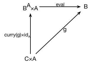
, there is a unique function (arrow) \text{curry}(g) that makes the following diagram commute

Now, how does all this relate to what we understand as currying?

It shows us that in category theory we can have an object that is effectively represents a function type in the same category as the object that represents the type of values it operates on, and you can capture the notion of applying values of that function type onto values of their parameter type using an arrow.

As I said before: not every category has a structure that can support exponentiation. The examples of this aren’t particularly easy to follow. The easiest one I’ve found is Top the category of topological spaces. In Top, the exponent doesn’t exist for many objects. Objects in Top are topological spaces, and arrows are continuous functions between them. For any two objects in Top, you can create the necessary objects for the exponential. But for many topological spaces, the required arrows don’t exist. The functions that they correspond to exist in Set, but they’re not continuous – and so they aren’t arrows in Top. (The strict requirement is that for an exponential X^Y to exist, Y must be a locally compact Hausdorff space. What that means is well beyond the scope of this!)

Cartesian Closed Categories

If you have a category C, and for every pair of objects A and B in the category C, there exists an exponential object B^A \in C, then we’ll say that C has exponentiation. Similarly, if for every pair of objects A, B \in Ob(C), there exists a product object A\times B, we say that the category has products.
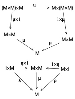
There’s a special kind of category, called a cartesian closed category, which is a category  where:

  1. Every pair of objects has both product and exponent objects; and
  2. Which has at least one terminal object. (Remember that terminals are something like singletons, and so they work as a way of capturing the notion of being a single element of an object; so this requirement basically says that the category has at least one value that “functions” can be applied to.)

That may seem like a very arbitrary set of rules: what’s so important about having all products, exponents, and a terminal object?

It means that we have a category which can model types, functions, and function application. Lambda calculus proves that that’s all you need to model computation. Closed cartesian categories are, basically, a formal model of a computing system! Any cartesian closed category is a model for a simply typed \lambda-calculus; and \lambda-calculus is something known as the internal language of a cartesian closed category.

What “internal language” means formally is complicated, but in simple terms: you can take any computation in lambda calculus, and perform the computation by chasing arrows in a category diagram of a closed cartesian category that includes the values of that calculus. Alternatively, every computation step that you perform evaluating a \lambda-calculus expression corresponds to an arrow in a CCC.

References

For this post, I’ve made heavy use of:

Another Stab at Category Theory: Lesson one: Starting with Monoids

Introduction and Motivation

One thing that I keep bumping up against as an engineer who loves functional a programming is category theory. It often seems like there are two kinds of functional programmers: people who came into functional programming via engineering, and people who came into functional programming via math. The problem is that a lot of the really interesting work in languages and libraries for functional programming are being built from the mathematical side, but for people on the engineering side, it’s impenetrable: it’s like it’s written in a whole different language, and even basic discussions about programming go off the rails, because the basic abstractions don’t make any sense if you don’t know category theory.

But how do you learn category theory? It seems impenetrable to mere humans. For example, one of the textbooks on category theory that several people told me was the most approachable starts chapter one with the line:

A group extension of an abelian group H by an abelian group G consists of a group E together with an inclusion of G \hookrightarrow E as a normal subgroup and a surjective homomorphism E \twoheadrightarrow H that displays H as the quotient group E|G.

If you’re not a professional mathematician, then that is pure gobbledigook. But that seems to be typical of how initiates of category theory talk about it. But the basic concepts, while abstract, really aren’t all that tricky. In many ways, it feels a lot like set theory: there’s a simple conceptual framework, on which you can build extremely complicated formalisms. The difference is that while many people have spent years figuring out how to make the basics of set theory accessible to lay-people, but that effort hasn’t been applied to set theory.

What’s the point?

Ok, so why should you care about category theory?

Category theory is a different way of thinking, and it’s a language for talking about abstractions. The heart of engineering is abstraction. We take problems, and turn them into abstract structures. We look at the structures we create, and recognize commonalities between those structures, and then we create new abstractions based on the commonalities. The hardest part of designing a good library is identifying the right abstractions.

Category theory is a tool for talking about structures, which is particularly well suited to thinking about software. In category theory, we think in terms of arrows, where arrows are mappings between objects. We’ll see what that means in detail later, but the gist of it is that one example of arrows mapping between objects is functions mapping between data types in a computer program.

Category theory is built on thinking with orrows, and building structures using arrows. It’s about looking at mathematical constructions built with arrows, and in those structures, figuring out what the fundamental parts are. When we abstract enough, we can start to see that things that look very different are really just different realizations of the same underlying structure. Category theory gives us a language and a set of tools for doing that kind of abstraction – and then we can take the abstract structures that we identify, and turn them into code – into very generic libraries that express deep, fundamental structure.

Start with an Example: Monoids

Monoids in Code

We’ll get started by looking at a simple mathematical structure called a monoid, and how we can implement it in code; and then, we’ll move on to take an informal look at how it works in terms of categories.

Most of the categorical abstractions in Scala are implemented using something called a typeclass, so we’ll start by looking at typeclasses. Typeclasses aren’t a category theoretical notion, but they make it much, much easier to build categorical structures. And they do give us a bit of categorical flavor: a typeclass defines a kind of metatype – that is, a type of type – and we’ll see, that kind of self-reflective abstraction is a key part of category theory.

The easiest way to think about typeclasses is that they’re a kind of metatype – literally, as the name suggests, they define classes where the elements of those classes are types. So a typeclass provides an interface that a type must provide in order to be an instance of the metatype. Just like you can implement an interface in a type by providing implementations of its methods, you can implement a typeclass by providing implementations of its operations.

In Scala, you implement the operations of a typeclasses using a language construct called an implicit parameter. The implicit parameter attaches the typeclass operations to a meta-object that can be passed around the program invisibly, providing the typeclass’s operations.

Let’s take a look at an example. An operation that comes up very frequently in any kind of data processing code is reduction: taking a collection of values of some type, and combining them into a single value. Taking the sum of a list of integers, the product of an array of floats, and the concatenation of a list of strings are all examples of reduction. Under the covers, these are all similar: they’re taking an ordered group of values, and performing an operation on them. Let’s look at a couple of examples of this:

def reduceFloats(floats: List[Float]): Float =
    floats.foldRight(0)((x, y) => x + y)

def reduceStrings(strings: Seq[String]): String =
    strings.foldRight("")((x, y) => x.concat(y))

When you look at the code, they look very similar. They’re both just instantiations of the same structural pattern:

def reduceX(xes: List[X]): X =
    xes.foldRight(xIdentity)((a, b) => Xcombiner(a, b))

The types are different; the actual operation used to combine the values is different; the base value in the code is different. But they’re both built on the same pattern:

  • There’s a type of values we want to combine: Float or String. Everything we care about in reduction is a connected with this type.
  • There’s a collection of values that we want to combine, from left to right. In one case, that’s a List[Float], and in the other, it’s a Seq[String]. The type doesn’t matter, as long as we can iterate over it.
  • There’s an identity value that we can use as a starting point for building the result; 0 for the floats, and "" (the empty string) for the strings.
  • There’s an operation to combine two values: + for the floats, and concat for the strings.

We can capture that concept by writing an interface (a trait, in Scala terms) that captures it; that interface is called a typeclass. It happens that this concept of reducible values is called a monoid in abstract algebra, so that’s the name we’ll use.

trait Monoid[A]  {
    def empty: A
    def combine(x: A, y: A): A
}

We can read that as saying “A is a monoid if there are implementations of empty and combine that meet these constraints”. Given the declaration of the typeclass, we can implement it as an object which provides those operations for a particular type:

object FloatAdditionMonoid extends Monoid[Float] {
    def empty: Float = 0.0
    def combine(x: Float, y: Float): Float = x + y
}

object StringConcatMonoid extends Monoid[String] {
    def empty: String = ""
    def combine(x: String, y: String): String = x.concat(y)
}

FloatAdditionMonoid implements the typeclass Monoid for the type Float. And since we can write an implementation of Monoid for Float or String, we can say that the types Float and String are instances of the typeclass Monoid.

Using our implementation of Monoid, we can write a single, generic reduction operator now:

def reduce[A](values: Seq[A], monoid: Monoid[A]): A =
   values.foldRight(monoid.empty)(monoid.combine)

We can use that to reduce a list of floats:

reduce([1.0, 3.14, 2.718, 1.414, 1.732], FloatAdditionMonoid)

And we can do a bit better than that! We can set up an implicit, so that we don’t need to pass the monoid implementation around. In Scala, an implicit is a kind of dynamically scoped value. For a given type, there can be one implicit value of that type in effect at any point in the code. If a function takes an implicit parameter of that type, then the nearest definition in the execution stack will automatically be inserted if the parameter isn’t passed explicitly.

def reduce[A](values: Seq[A])(implicit A: Monoid[A]): A =
   list.foldRight(A.empty)(A.combine)

And as long as there’s a definition of the Monoid for a type A in scope, we can can use that now by just writing:

implicit object FloatAdditionMonoid extends Monoid[Float] {
    def empty: Float = 0.0
    def combine(x: Float, y: Float): Float = x + y
}

val floats: List[Float] = ...
val result = reduce(floats)

Now, anywhere that the FloatAdditionMonoid declaration is imported, you can call reduce on any sequence of floats, and the implicit value will automatically be inserted.

Using this idea of a monoid, we’ve captured the concept of reduction in a common abstraction. Our notion of reduction doesn’t care about whether we’re reducing strings by concatenation, integers by addition, floats by multiplication, sets by union. Those are all valid uses of the concept of a monoid, and they’re all easy to implement using the monoid typeclass. The concept of monoid isn’t a difficult one, but at the same time, it’s not necessarily something that most of us would have thought about as an abstraction.

We’ve got a typeclass for a monoid; now, we’ll try to connect it into category theory. It’s a bit tricky, so we won’t cover it all at once. We’ll look at it a little bit now, and we’ll come back to it in a later lesson, after we’ve absorbed a bit more.

From Sets to Arrows

For most of us, if we’ve heard of monoids, we’ve heard of them in terms of set theory and abstract algebra. So in that domain, what’s a monoid?

A monoid is a triple (V, 1, *), where:

  • V is a set of values;
  • 1 is a value in V;
  • * is a total binary operator where:
    • 1 is an identity of *: For any value v \in V: v*1 = 1*v = v.
    • * is associative: for any values v, w, x \in V: (v * w) * x = v * (w * x)

That’s all just a formal way of saying that a monoid is a set with a binary associative operator and an identity value. The set of integers can form a monoid with addition as the operator, and 0 as identity. Real numbers can be a monoid with multiplication and 1. Strings can be a monoid with concatenation as the operator, and empty string as identity.

But we can look at it in a different way, too, by thinking entirely in terms of function.
Let’s forget about the numbers as individual values, and instead, let’s think about them in functional terms. Every number is a function which adds itself to its parameter. So “2” isn’t a number, it’s a function which adds two to anything.

How can we tell that 2 is a function which adds two to things?

If we compose it with 3 (the function that adds three to things), we get 5 (the function that adds five to things). And how do we know that? Because it’s the same thing that we get if we compose 3 with 1, and then compose the result of that with 1 again. 3+1+1=5, and 3+2=5. We can also tell that it’s 2, because if we just take 1, and compose it with itself, what we’ll get back is the object that we call 2.

In this scheme, all of the numbers are related not by arithmetic, not by an underlying concept of quantity or cardinality or ordinality, but only by how they compose with each other. We can’t see anything else – all we have are these functions. But we can recognize that they are the natural numbers that we’re familiar with.

Looking at it this way, we can think of the world of natural numbers as a single point, which represents the set of all natural numbers. And around that point, we’ve got lots and lots of arrows, each of which goes from that point back to itself. Each of those arrows represents one number. The way we tell them apart is by understanding which arrow we get back when we compose them. Take any arrow from that point back to that point, and compose it with the arrow 0, and what do you get? The arrow you started with. Take any arrow that you want, and compose it with 2. What do you get? You get the same thing that you’d get if you composed it with 1, and then composed it with one again.

That dot, with those arrows, is a category.

What kind of advantage do we get in going from the algebraic notion of a set with a binary operation, to the categorical notion of an object with a bunch of composable arrows? It allows to understand a monoid purely as a structure, without having the think about what the objects are, or what the operator means.

Now, let’s jump back to our monoid typeclass for a moment.

trait Monoid[A]  {
    def empty: A
    def combine(x: A, y: A): A
}

We can understand this as being a programmable interface for the categorical object that we just described. All we need to do is read “:” as “is an arrow in”: It says that A is a monoid if:

  • It has an element called empty which is an arrow in A.
  • It has an operation called combine which, given any two arrows in A, composes them into a new arrow in A.

There are, of course, other conditions – combine needs to be associative, and empty needs to behave as the identity value. But just like when we write an interface for, say, a binary search tree, the interface only defines the structure not the ordering condition, the typeclass defines the functional structure of the categorical object, not the logical conditions.

This is what categories are really all about: tearing things down to a simple core, where everything is expressed in terms of arrows. It’s almost reasoning in functions, except that it’s even more abstract than that: the arrows don’t need to be functions – they just need to be composable mappings from things to things.

Deeper Into Arrows

We can abstract a bit more, and look at the entire construction, including the identity and associativity constraints entirely in terms of arrows. To really understand this, we’ll need to spend some time diving deeper into the actual theory of categories, but as a preview, we can describe a monoid with the following pair of diagrams (copied from wikipedia):

In these diagrams, any two paths between the same start and end-nodes are equivalent (up to isomorphism). When you understand how to read this diagrams, these really do define everything that we care about for monoids.

For now, we’ll just run through and name the parts – and then later, in another lesson, we’ll come back, and we’ll look at this in more detail.

  • \mu is an arrow from M\times M \rightarrow M, which we’ll call a multiplication operator.
  • \eta is an arrow from I \rightarrow M, called unit.
  • \alpha is an arrow from (M\times M)\times M \rightarrow M \times (M\times M) which represents the associativity property of the monoid.
  • \lambda is a morphism which represents the left identity property of the monoid (that is, 1*x=x), and \rho is a morphism representing the right identity property (x*1=x).

This diagram, using these arrows, is a way of representing all of the key properties of a monoid via nothing but arrows and composition. It says, among other things, that:

  • (M \times M) \times M composes with multiplication to be M \times M.
    That is, applying multiplication to (M \times M) \times M evaluates to (M \times M).
  • (M \times M) \times M composed with associativity can become M \times (M \times M).

So it’s a monoid – but it’s a higher level monoid. In this, M isn’t just an object in a category: it’s an entire category. These arrows are arrows between categories in a category of categories.

What we’ll see when we get deeper into category theory is how powerful this kind of abstraction can get. We’ll often see a sequence of abstractions, where we start with a simple concept (like monoid), and find a way to express it in terms of arrows between objects in a category. But then, we’ll lift it up, and look at how we can see in not just as a relation between objects in a category, but as a different kind of relation between categories, by constructing the same thing using a category of categories. And then we’ll abstract even further, and construct the same thing using mappings between categories of categories.

(You can find the next lesson <a href=”http://www.goodmath.org/blog/2019/02/20/category-theory-lesson-2-basics-of-categorical-abstraction/”>here</a>.)

Understanding Global Warming Scale Issues

Aside from the endless stream of Cantor cranks, the next biggest category of emails I get is from climate “skeptics”. They all ask pretty much the same question. For example, here’s one I received today:

My personal analysis, and natural sceptisism tells me, that there are something fundamentally wrong with the entire warming theory when it comes to the CO2.

If a gas in the atmosphere increase from 0.03 to 0.04… that just cant be a significant parameter, can it?

I generally ignore it, because… let’s face it, the majority of people who ask this question aren’t looking for a real answer. But this one was much more polite and reasonable than most, so I decided to answer it. And once I went to the trouble of writing a response, I figured that I might as well turn it into a post as well.

The current figures – you can find them in a variety of places from wikipedia to the US NOAA – are that the atmosphere CO2 has changed from around 280 parts per million in 1850 to 400 parts per million today.

Why can’t that be a significant parameter?

There’s a couple of things to understand to grasp global warming: how much energy carbon dioxide can trap in the atmosphere, and hom much carbon dioxide there actually is in the atmosphere. Put those two facts together, and you realize that we’re talking about a massive quantity of carbon dioxide trapping a massive amount of energy.

The problem is scale. Humans notoriously have a really hard time wrapping our heads around scale. When numbers get big enough, we aren’t able to really grasp them intuitively and understand what they mean. The difference between two numbers like 300 and 400ppm is tiny, we can’t really grasp how in could be significant, because we aren’t good at taking that small difference, and realizing just how ridiculously large it actually is.

If you actually look at the math behind the greenhouse effect, you find that some gasses are very effective at trapping heat. The earth is only habitable because of the carbon dioxide in the atmosphere – without it, earth would be too cold for life. Small amounts of it provide enough heat-trapping effect to move us from a frozen rock to the world we have. Increasing the quantity of it increases the amount of heat it can trap.

Let’s think about what the difference between 280 and 400 parts per million actually means at the scale of earth’s atmosphere. You hear a number like 400ppm – that’s 4 one-hundreds of one percent – that seems like nothing, right? How could that have such a massive effect?!

But like so many other mathematical things, you need to put that number into the appropriate scale. The earths atmosphere masses roughly 5 times 10^21 grams. 400ppm of that scales to 2 times 10^18 grams of carbon dioxide. That’s 2 billion trillion kilograms of CO2. Compared to 100 years ago, that’s about 800 million trillion kilograms of carbon dioxide added to the atmosphere over the last hundred years. That’s a really, really massive quantity of carbon dioxide! scaled to the number of particles, that’s something around 10^40th (plus or minus a couple of powers of ten – at this scale, who cares?) additional molecules of carbon dioxide in the atmosphere. It’s a very small percentage, but it’s a huge quantity.

When you talk about trapping heat, you also have to remember that there’s scaling issues there, too. We’re not talking about adding 100 degrees to the earths temperature. It’s a massive increase in the quantity of energy in the atmosphere, but because the atmosphere is so large, it doesn’t look like much: just a couple of degrees. That can be very deceptive – 5 degrees celsius isn’t a huge temperature difference. But if you think of the quantity of extra energy that’s being absorbed by the atmosphere to produce that difference, it’s pretty damned huge. It doesn’t necessarily look like all that much when you see it stated at 2 degrees celsius – but if you think of it terms of the quantity of additional energy being trapped by the atmosphere, it’s very significant.

Calculating just how much energy a molecule of CO2 can absorb is a lot trickier than calculating the mass-change of the quantity of CO2 in the atmosphere. It’s a complicated phenomenon which involves a lot of different factors – how much infrared is absorbed by an atom, how quickly that energy gets distributed into the other molecules that it interacts with… I’m not going to go into detail on that. There’s a ton of places, like here, where you can look up a detailed explanation. But when you consider the scale issues, it should be clear that there’s a pretty damned massive increase in the capacity to absorb energy in a small percentage-wise increase in the quantity of CO2.

Godel part 2: Arithmetic and Logic

In the last post, we saw how to take statements written in the logic of the Principia Mathematica, and convert them into numerical form using Gödel numbering. For the next step in Gödel’s proof, we need to go meta-mathematical.

Ultimately, we want to write first-order statements that can reason about first order statements. But the entire structure of the principia and its logic is designed to make
that impossible. First order statements can only reason about numbers and their properties.

But now, we’ve got the ability to represent statements – first order, second order, third order, any order. What we still need is a way of describing the properties of those numerical statements in terms of operations that can be expressed using nothing but first order statements.

The basic trick to incompleteness is that we’re going to use the numerical encoding of statements to say that a predicate or relation is represented by a number. Then we’re going to write predicates about predicates by defining predicates on the numerical representations of the first-order predicates. That’s going to let us create a true statement in the logic that can’t be proven with the logic.

To do that, we need to figure out how to take our statements and relations represented as numbers, and express properties of those statements and relations in terms of arithmetic. To do that, we need to define just what it means to express something arithmetically. Gödel did that by defining “arithmetically” in terms of a concept called primitive recursion.

I learned about primitive recursion when I studied computational complexity. Nowadays, it’s seen as part of theoretical computer science. The idea, as we express it in modern terms, is that there are many different classes of computable functions. Primitive recursion is one of the basic complexity classes. You don’t need a Turing machine to compute primitive recursive functions – they’re a simpler class.

The easiest way to understand primitive recursion is that it’s what you get in a programming language with integer arithmetic, and simple for-loops. The only way you can iterate is by repeating things a bounded number of times. Primitive recursion has a lot of interesting properties: the two key ones for our purposes here are: number theoretic proofs are primitive recursive, and every computation of a primitive recursive function is guaranteed to complete within a bounded amount of time.

The formal definition of primitive recursion, the way that Gödel wrote it, is quite a bit more complex than that. But it means the same thing.

We start with what it means to define a formula via primitive recursion. (Note the language that I used there: I’m not explaining what it means for a function to be primitive recursive; I’m explaining what it means to be defined via primitive recursion.) And I’m defining formulae, not functions. In Gödel’s proof, we’re always focused on numerical reasoning, so we’re not going to talk about programs or algorithms, we’re going to about the definition of formulae.

A formula phi(x_1, x_2, ..., x_n) is defined via primitive recursion if, for some other formulae \psi and \mu:

  • Base: \phi(0, x_2, ..., x_n) = \psi(x_2, ..., x_n)
  • Recursive: \phi(i+1, x_2, ..., x_n) = \mu(i, \phi(i, x_2, ..., x_n), x_2, ..., x_n).

So, basically, the first parameter is a bound on the number of times that phi can invoked recursively. When it’s 0, you can’t invoke \phi any more.

A formula is primitive recursive if it defined from a collection of formulae \phi_1, ..., \phi_n where any formula \phi_i is defined via primitive recursion from \phi_1, ..., \phi_{i-1}, or the primitive succ function from Peano arithmetic.

For any formula phi_i in that sequence, the degree of the formula is the number of other primitive recursive formulae used in its definition.

Now, we can define a primitive recursive property: R(x_1, ..., x_n) is primitive recursive if and only if there exists a primitive recursive function \phi such that \phi(x_1, ..., x_n) = 0.

With primitive recursive formulae and relations defined, there’s a bunch of theorems about how you can compose primitive recursive formulae and relations:

  1. Every function or relation that you get by substituting a primitive recursive function for a variable in a primitive recursive function/relation is primitive recursive.
  2. If R and S are primitive relations, then ¬R, R∧S, R∨S are all primitive recursive.
  3. If \phi(x_1, ..., x_n) and \psi(x_1, ..., x_n) are primitive recursive functions, then the relation R(x_1, ..., x_n) \Leftrightarrow (\phi(x_1, ..., x_n) = \psi(x_1, ..., x_n) is also primitive recursive.
  4. Let xv and zv be finite-length tuples of variables. If the function \phi(xv) and the relation R(y, zv) are primitive recursive, then so are the relations:
    • S(xv, zv) \Leftrightarrow  (\exists y \le \phi(xv). R(y, zv))
    • T(xv, zv) \Leftrightarrow  (\forall y \le A(xv). R(y, zv))
  5. Let xv and zv be finite-length tuples of variables. And let text{argmin}[y le f(x).R(x)] be the smallest value of x for which y le f(x) and R(x) is true, or 0 if there is no such value. Then if the function phi(xv) and the relation R(y, zv) are primitive recursive, then so is the function P(xv, zv) = (\text{argmin}[y \le A(xv). R(y, zv))].

By these definitions, addition, subtraction, multiplication, and integer division are all primitive recursive.

Ok. So, now we’ve got all of that out of the way. It’s painful, but it’s important. What we’ve done is come up with a good formal description of what it means for something to be an arithmetic property: if we can write it as a primitive recursive relation or formula, it’s arithmetic.