
In the stuff I’ve been writing about topology so far, I’ve been talking about topologies mostly algebraically. I’m not sure why, but for me, algebraic topology is both the most interesting and easy to understand bit of topology. Most people seem to think I’m crazy; in general, people seem to think that algebraic topology is hard. It must say something about me that I find other things much harder, but I’ll leave it to someone else to figure out what.
Despite the fact that I love the algebraic side, there’s a lot of interesting stuff in topology that you need to talk about, which isn’t purely algebraic. Today I’m going to talk about one of the most important ones: manifolds.
The definition we use for topological spaces is really abstract. A topological space is a set of points with a structural relation. You can define that relation either in terms of neighborhoods, or in terms of open sets – the two end up being equivalent. (You can define the open sets in terms of neighborhoods, or the neighborhoods in terms of open sets; they define the same structure and imply each other.)
That abstract definition is wonderful. It lets you talk about lots of different structures using the language and mechanics of topology. But it is very abstract. When we think about a topological space, we’re usually thinking of something much more specific than what’s implied by that definition. The word space has an intuitive meaning for us. We hear it, and we think of shapes and surfaces. Those are properties of many, but not all topological spaces. For example, there are topological spaces where you can have multiple distinct points with identical neighborhoods. That’s definitely not part of what we expect!
The things that we think of as a spaces are really are really a special class of topological spaces, called manifolds.
Informally, a manifold is a topological space where its neighborhoods for a surface that appears to be euclidean if you look at small sections. All euclidean surfaces are manifolds – a two dimensional plane, defined as a topological space, is a manifold. But there are also manifolds that aren’t really euclidean, like a torus, or the surface of a sphere – and they’re the things that make manifolds interesting.
The formal definition is very much like the informal, with a few additions. But before we get there, we need to brush up on some definitions.
- A set
is countable if and only if there is a total, onto, one-to-one function from
- Given a topological space
, a basis
for
is a collection of open sets from which any open set in
- A topological space
, there are at least one open set
where
, and at least one open set
where
. (That is, there is at least one open set that includes
but not
, and one that includes
A topological space
-
-
- Every point in
has a neighborhood homeomorphic to an open euclidean
-ball.
Basically, what this really means is pretty much what I said in the informal definition. In a euclidean
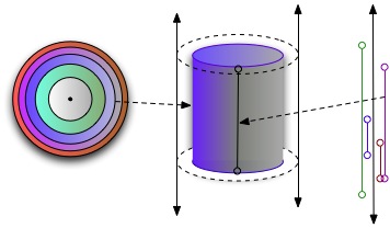
If you think of a large enough torus, you can easily imagine that the smaller open 2-balls (disks) around a particular point will look very much like flat disks. In fact, as the torus gets larger, they’ll become virtually indistinguishable from flat euclidean disks. But as you move away from the individual point, and look at the properties of the entire surface, you see that the euclidean properties fail.
Another interesting way of thinking about manifolds is in terms of a construction called charts, and charts will end up being important later.
A chart for an manifold is an invertable map from some euclidean manifold to part of the manifold which preserves the topological structure. If a manifold isn’t euclidean, then there isn’t a single chart for the entire manifold. But we can find a set of overlapping charts so that every point in the manifold is part of at least one chart, and the edges of all of the charts overlap. A set of overlapping charts like that is called an atlas for the manifold, and we will sometimes say that the atlas defines the manifold. For any given manifold, there are many different atlases that can define it. The union of all possible atlases for a manifold, which is the set of all charts that can be mapped onto parts of the manifold is called the maximal atlas for the manifold. The maximal atlas for a manifold is, obviously, unique.
For some manifolds, we can define an atlas consisting of charts with coordinate systems. If we can do that, then we have something wonderful: a topology on which we can do angles, distances, and most importantly, calculus.
Topologists draw a lot of distinctions between different kinds of manifolds; a few interesting examples are:
- A Reimann manifold is a manifold on which you can meaningfully define angles and distance. (The mechanics of that are complicated and interesting, and I’ll talk about them in a future post.)
- A differentiable manifold is one on which you can do calculus. (It’s basically a manifold where the atlas has measures, and the measures are compatible in the overlaps.) I probably won’t say much more about them, because the interesting thing about them is analysis, and I stink at analysis.
- A Lie group is a differentiable manifold with a valid closed product operator between points in the manifold, which is compatible with the smooth structure of the manifold. It’s basically what happens when a differentiable manifold and a group fall in love and have a baby.
We’ll see more about manifolds in future posts!
 and
and  . Both
  to a topological space
  . What does it mean to say that the function
 ![U = [0, 1]](http://l.wordpress.com/latex.php?latex=U%20%3D%20%5B0%2C%201%5D&bg=FFFFFF&fg=000000&s=0 "U = [0, 1]") .
. , where
  = f(a) \land t(a, 1) = g(a)") .
.  is a homotopy between
  and
and  are continuous functions, then the spaces
  is homotopic with the id function on
  is homotopic with the id function on
  is defined as the set of all possible pairs
 ") , where
, where  and
and  . If
. If  and
and  , then
 , (1, 5), (2, 4), (2, 5), (3, 4), (3, 5) \}") .
. of objects, and two functions
  and
and  . (To be complete, we’d need to add some conditions, but the idea should be clear from this much.) Given any object in the the product set
 ") will give us the projection of that object onto
will give us the projection of that object onto  and
and  .
.  in
in ") is an open-set in
is an open-set in 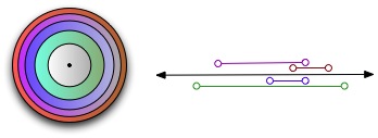
") , where
, where  is a set of objects, called points;
  is a function from elements of
 : p \in A") : every neighborhood of a point must include that point.
: every neighborhood of a point must include that point.: \forall B \in X: B \supset A \Rightarrow B \in N(p)") . If
. If : A \cap B \in N(p)") : the intersection of any two neighborhoods of a point is a neighborhood of that point.
: the intersection of any two neighborhoods of a point is a neighborhood of that point.: \exists B \in N(x): \forall b \in B: A \in N(b)") . If
. If  is if
is if  < d(q, r)") .)
.) = d(r, p)") .)
.)") of a point are equivalent to the open balls around
of a point are equivalent to the open balls around ") and
and ") are both topological spaces, then a function
are both topological spaces, then a function  is continuous if and only if for every open set
  , the inverse image of
  is an open set in
  . (The inverse image of
  \in C") ).
).") and
and ") are close together in
are close together in  , then
  and
and  must have been close together in
  are continuous.
 = \sqrt{(x_2-x_1)^2 + (y_2-y_1)^2}")
 is a distance metric if it satisfies the following requirements:
 = 0 \Leftrightarrow s_i = s_j")
 = d(s_j, s_i)")
 \le d(s_i, s_j) + d(s_j, s_k)")
 \ge 0")
") of a set
of a set  over the set. For example:
, (b_x,b_y)) = \sqrt{(a_x-b_x)^2 + (a_y-b-y)^2}") .
.") , and a point
, and a point  . An open ball B(p, r) (that is, a ball of radius
  < r") .
., B(p, 2\epsilon), B(p, 3\epsilon)") , and so on. Once you’ve got that series of ever-smaller and ever-larger open balls around a point
, and so on. Once you’ve got that series of ever-smaller and ever-larger open balls around a point