I’m a nice jewish boy, so I grew up eating a lot of brisket. Brisket’s an interesting
piece of meat. By almost any reasonable standard, it’s an absolutely godawful cut
of beef. It’s ridiculously tough. We’re not talking just a little bit chewy here: you can
cook a hunk of brisket for four hours, still have something that’s inedible, because your
teeth can’t break it down. It’s got a huge layer of fat on top – but the meat itself is
completely lean – so if you cook it long enough to be chewable, it can be dry as a bone.
But my ancestors were peasants. They couldn’t afford to eat beef normally, and when
special occasions rolled around, the only beef they could afford was the stuff that
no one else wanted. So they got briskets.
If you get interested in foods, though, you learn that many of the best foods in the world started off with some poor peasant who wanted to make something delicious, but couldn’t afford expensive ingredients! Brisket is a perfect example. Cook it for a good long time,
or in a pressure cooker, with lots of liquid, and lots of seasoning, and it’s one of
the most flavorful pieces of the entire animal. Brisket is really delicious,
once you manage to break down the structure that makes it so tough. These days, it’s
become super trendy, and everyone loves brisket!
Anyway, like I said, I grew up eating jewish brisket. But then I married a Chinese woman, and in our family, we always try to blend traditions as much as we can. In particular, because we’re both food people, I’m constantly trying to take things from my tradition, and blend some of her tradition into it. So I wanted to find a way of blending some chinese flavors into my brisket. What I wound up with is more japanese than chinese, but it works. The smoky flavor of the dashi is perfect for the sweet meatiness of the brisket, and the onions slowly cook and sweeten, and you end up with something that is distinctly similar to the traditional jewish onion-braised-brisket, but also very distinctly different.
Ingredients:
1 brisket.
4 large onions.
4 packets of shredded bonito flakes from an asian market.
4 large squares of konbu (japanese dried kelp)
1 cup soy sauce.
1 cup apple cider.
Random root vegetables that you like. I tend to go with carrots
and daikon radish, cut into 1 inch chunks.
Instructions
First, make some dashi:
Put about 2 quarts of water into a pot on your stove, and bring to a boil.
Lower to a simmer, and then add the konbu, and simmer for 30 minutes.
Turn off the heat, add the bonito, and then let it sit for 10 minutes.
Strain out all of the kelp and bonito, and you’ve got dashi!.
Slice all of the onions into strips.
Cut the brisket into sections that will fit into an instant pot or other pressure cooker.
Fill the instant pot by laying a layer of onions, followed by a piece of brisket, followed by a layer of onions until all of the meat is covered in onions.
Take your dashi, add the apple cider, and add soy sauce until it tastes too salty. That’s just right (Remember, your brisket is completely unsalted!) Pour it over the brisket and onions.
Fill in any gaps around the brisket and onions with your root vegetables.
Cook in the instant pot for one hour, and then let it slowly depressurize.
Meanwhile, preheat your oven to 275.
Transfer the brisket from the instant pot to a large casserole or dutch oven. Cover with the onions. Taste the sauce – it should be quite a bit less salty. If it isn’t salty enough, add a bit more sauce sauce; if it tastes sour, add a bit more apply cider.
Cook in the oven for about 1 hour, until the top has browned; then turn the brisket over, and let it cook for another hour until the other side is brown.
Slice into thick slices. (It should be falling apart, so that you can’t cut it thin!).
Strain the fat off of the broth, and cook with a bit of cornstarch to thicken into a gravy.
Quick personal aside: I haven’t been posting a lot on here lately. I keep wanting to get back to it; but each time I post anything, I’m met by a flurry of crap: general threats, lawsuit threats, attempts to steal various of my accounts, spam to my contacts on linkedin, subscriptions to ashley madison or gay porn sites, etc. It’s pretty demotivating. I shouldn’t let the jerks drive me away from my hobby of writing for this blog!
I started this series of posts by saying that Category Theory was an extremely abstract field of mathematics which was really useful in programming languages and in particular in programming language type systems. We’re finally at one of the first places where you can really see how that’s going to work.
If you program in Scala, you might have encountered curried functions. A curried function is something that’s in-between a one-parameter function and a two parameter function. For a trivial example, we could write a function that adds two integers in its usual form:
def addInt(x: Int, y: Int): Int = x + y
That’s just a normal two parameter function. Its curried form is slightly different. It’s written:
def curriedAddInt(x: Int)(y: Int): Int = x +y
The curried version isn’t actually a two parameter function. It’s a shorthand for:
def realCurrentAddInt(x: Int): (Int => Int) = (y: Int) => x + y
That is: currentAddInt is a function which takes an integer, x, and returns a function which takes one parameter, and adds x to that parameter.
Currying is the operation of taking a two parameter function, and turning it into a one-parameter function that returns another one-parameter function – that is, the general form of converting addInt to realAddInt. It might be easier to read its type: realCurrentAddInt: Int => (Int => Int): It’s a function that takes an int, and returns a new function from int to int.
So what does that have to do with category theory?
One of the ways that category theory applies to programming languages is that types and type theory turn out to be natural categories. Almost any programming language type system is a category. For example, the figure below shows a simple view of a programming language with the types Int, Bool, and Unit. Unit is the initial object, and so all of the primitive constants are defined with arrows from Unit.
For the most part, that seems pretty simple: a type T is an object in the programming language category; a function implemented in the language that takes a parameter of type A and returns a value of type B is an arrow from A to B. A multi-parameter function just uses the cartesian product: a function that takes (A, B) and returns a C is an arrow from .
But how could we write the type of a function like our curried adder? It’s a function from a value to a function. The types in our language are objects in the category. So where’s the object that represents functions from A to B?
As we do often, we’ll start by thinking about some basic concepts from set theory, and then generalize them into categories and arrows. In set theory, we can define the set of functions from to as: – that is, as exponentiation of the range of the produced functions.
There’s a product object .
There’s an arrow from , which we’ll call eval.
In terms of the category of sets, what that means is:
You can create a pair of a function from and an element of .
There is a function named eval which takes that pair, and returns an instance of .
Like we saw with products, there’s a lot of potential exponential objects which have the necessary product with , and arrow from that product to . But which one is the ideal exponential? Again, we’re trying to get to the object with thie universal property – the terminal object in the category of pseudo-exponentials. So we use the same pattern as before. For any potential exponential, there’s an arrow from the potential exponential to the actual exponential, and the potential exponential with arrows from every other potential exponential is the exponential.
Let’s start putting that together. A potential exponential for is an object where the following product and arrow exist:
There’s an instance of that pattern for the real exponential:
We can create a category of these potential exponentials. In that category, there will be an arrow from every potential exponential to the real exponential. Each of the potential exponentials has the necessary property of an exponential – that product and eval arrow above – but they also have other properties.
In that category of potential exponentials of , there’s an arrow from an object to an object if the following conditions hold in the base category:
There is an arrow in the base category.
There is an arrow
It’s easiest to understand that by looking at what it means in Set:
We’ve got sets and , which we believe are potential exponents.
has a function .
has a function .
There’s a function which converts a value of to a value of , and a corresponding function , which given a pair transforms it into a pair , where evaluating . In other words, if we restrict the inputs to to be effectively the same as the inputs to , then the two eval functions do the same thing. (Why do I say restrict? Because might have a larger domain than the range of , but these rules won’t capture that.)
An arrow in the category of potential products is a pair of two arrows in the base category: one from , and one from . Since the two arrows are deeply related (they’re one arrow in the category of potential exponentials), we’ll call them and . (Note that we’re not really taking the product of an arrow here: we haven’t talked about anything like taking products of arrows! All we’re doing is giving the arrow a name that helps us understand it. The name makes it clear that we’re not touching the right-hand component of the product.)
Since the exponential is the terminal, which means that that pair of curry arrows must exist for every potential exponential to the true exponential. So the exponential object is the unique (up to isomorphism) object for which the following is true:
There’s an arrow . Since is the type of functions from to , represents the application of one of those functions to a value of type to produce a result of type .
For each two-parameter function , there is a unique function (arrow) that makes the following diagram commute
Now, how does all this relate to what we understand as currying?
It shows us that in category theory we can have an object that is effectively represents a function type in the same category as the object that represents the type of values it operates on, and you can capture the notion of applying values of that function type onto values of their parameter type using an arrow.
As I said before: not every category has a structure that can support exponentiation. The examples of this aren’t particularly easy to follow. The easiest one I’ve found is Top the category of topological spaces. In Top, the exponent doesn’t exist for many objects. Objects in Top are topological spaces, and arrows are continuous functions between them. For any two objects in Top, you can create the necessary objects for the exponential. But for many topological spaces, the required arrows don’t exist. The functions that they correspond to exist in Set, but they’re not continuous – and so they aren’t arrows in Top. (The strict requirement is that for an exponential to exist, must be a locally compact Hausdorff space. What that means is well beyond the scope of this!)
Cartesian Closed Categories
If you have a category , and for every pair of objects and in the category , there exists an exponential object , then we’ll say that has exponentiation. Similarly, if for every pair of objects , there exists a product object , we say that the category has products.
There’s a special kind of category, called a cartesian closed category, which is a category where:
Every pair of objects has both product and exponent objects; and
Which has at least one terminal object. (Remember that terminals are something like singletons, and so they work as a way of capturing the notion of being a single element of an object; so this requirement basically says that the category has at least one value that “functions” can be applied to.)
That may seem like a very arbitrary set of rules: what’s so important about having all products, exponents, and a terminal object?
It means that we have a category which can model types, functions, and function application. Lambda calculus proves that that’s all you need to model computation. Closed cartesian categories are, basically, a formal model of a computing system! Any cartesian closed category is a model for a simply typed -calculus; and -calculus is something known as the internal language of a cartesian closed category.
What “internal language” means formally is complicated, but in simple terms: you can take any computation in lambda calculus, and perform the computation by chasing arrows in a category diagram of a closed cartesian category that includes the values of that calculus. Alternatively, every computation step that you perform evaluating a -calculus expression corresponds to an arrow in a CCC.
I’ve been thinking about how to talk about social anxiety more. This recently came up at work, and I thought it would be worth writing down. As usual, I’m talking about my own experiences as a person with severe social anxiety. I think there are others who feel the same way as I do – but equally, there are plenty of people with social anxiety disorders who feel very different. I can only talk about what I feel, and what I experience – so don’t assume that I’m talking for anyone but myself.
One of the interesting facets of social anxiety is that people
with SA don’t necessarily act the way that you expect us to. People
generally expect us to be like one of the characters from the Big
Bang theory.
In reality, most of us have an adaptive behavior that we learn,
which I call masking. For many people with social anxiety,
if you encounter them at work or on the street, you’d never guess
that we had any kind of anxiety problem. It’s the nature of social anxiety
that we want to hide the anxiety that we feel, and so we find ways to do it.
The heart of social anxiety for is the feeling that there’s
something wrong with me – that I’m weird, freakish, abnormal, that
I’m broken – and that when people realize that, they’re
going to reject me. It doesn’t make sense, but it doesn’t have to. I
can know, intellectually, that it’s a pile of crap, but that doesn’t
stop me from feeling it; it doesn’t stop my body from reacting to
it. I spent years of school being regularly abused – mocked, beaten,
tormented – and that got wired into my brain. That’s the way that I
expect to be treated by people I don’t know well – and even, sometimes,
by people that I do know.
A way to cope with that is to act like I’m a normal, functional
person. I don’t believe that I’m normal. I don’t really understand
what it’s like to be normal. But I’ve learned how, in many situation
to fake it well enough to get by. The way that I that is
masking. Think of what you do when you’re painting something. You
want to expose certain areas to the paint, and you don’t want to
expose others. So you cover up parts of the object with masking tape
– and then you’ll only get paint on the parts that aren’t
masked. That’s what I’ve learned to do. I to take a piece of myself
that I think is close to normal for a situation, and build a persona
around it. I mask off everything that doesn’t fit – so people can’t
see the parts of me that I don’t want them to. Masking makes it
much easier to interact, both because I’ve constructed the mask to
only show the parts of myself that I think people won’t react badly
to. I’ve created a version of myself that I hope won’t draw any
attention for being weird.
A mask lets me appear to be a normal, confident person. It lets me go
to work each day, and interact with people on the train, on the street,
in the office, without turning into a basket case from the stress.
I try to be open with the people I really work closely with about
who I am, and what I feel. I don’t hide the fact that I have social anxiety,
and I do my best to minimize the mask. But I do wear a mask at work,
because without it, I wouldn’t be able to function.
The people I work with think I’m kind-of loud. They think I’m really
confident – probably a bit over-confident. I try to talk about my social
anxiety disorder, but I’m not sure if they actually believe me – because
what I’m saying about how I feel isn’t consistent with how they see me
behave. My masks have gotten good enough that as long as I’m in a situation
that I’ve prepared for, most of the time, you can’t see past it to actually
see what I’m feeling.
The big weakness of a mask is that it’s an act. It’s not the real
me – it’s a face that present to the world so that they don’t really
see me. It’s something that I need to consciously construct and
prepare. If I’m put into a situation that I couldn’t prepare for,
then I don’t necessary have a mask ready. And that means that I’m
just me – the broken person who’s paralyzed with fear.
I can get up in front of a classroom full of people, and give a lecture.
I can get up in front of the congregation at my synagogue, and give a drash
that I wrote – I can do both of those things without feeling overly stressed.
People expect that a person with social anxiety won’t be able to do that,
but that’s easy. It’s a situation where I know what’s expected
of me, where I know what to do and how to behave. So I can mask myself
in a way that lets me show the parts of myself that I need for that
performance, and hide the rest.
But ask me to sit down and eat lunch with a random selection of
people after I’m done teaching my class? That is hard. I
don’t know who I’m dealing with. I don’t know how to talk to them,
what they expect from me, how they’re going to react to me. That’s
the kind of situation that triggers my anxiety, and that can,
easily, wreck me. I don’t have a mask ready for that.
In my last post about category theory, I introduced the basic idea of typeclasses, and showed how to implement an algebraic monoid as a typeclass. Then we used that algebraic monoid as an example of how to think with arrows, and built it up into a sketch of category theory’s definition of a monoid. We ended with an ominous looking diagram that illustrated what a categorical monoid looks like.
In this post, we’re going to take a look at some of the formal definitions of the basic ideas of category theory. By the end of this lesson, you should be able to look at the categorical monoid, and understand what it means. But the focus of this post will be on understanding initial and terminal objects, and the role they play in defining abstractions in category theory. And in the next post, we’ll see how abstractions compose, which is where the value of category theory to programmers will really become apparrent.
Before I really get started: there’s a lot of terminology in category theory, and this post has a lot of definitions. Don’t worry: you don’t need to remember it all. You do need to understand the concepts behind it, but specifically remembering the difference between, say, and endomorphism, and epimorphism, and a monomorphism isn’t important: you can always look it up. (And I’ll put together a reference glossary to help make that easy.)
Defining Categories
A category is basically a directed graph – a bunch of dots connected by arrows, where the arrows have to satisfy a bunch of rules.
Formally, we can say that a category consists of a the parts: , where:
is a collection of objects. We don’t actually care what the objects are – the only thing we can do in category theory is look at how the objects related through arrows that connect them. For a category , we’ll often call this collection Obj(C).
is a collection of arrows, often called morphisms. Each element of starts at one object called its domain (often abbreviated dom), and ending at another object called its codomain (abbreviated cod). For an arrow that goes from to , we’ll often write it as . For a category , we’ll often call this set Mor(C) (for morphisms of C).
is a composition operator. For every pair of arrows , and , there must be an arrow called the compositions of and .
To be a category, these must satisfy the following rules:
Identity: For every object , there must be an arrow from to , called the identity of . We’ll often write it as . For any arrow ; and for any arrow . That’s just a formal way of saying that composing an identity arrow with any other arrow results in the the other arrow.
Associativity: For any set of arrows .
When talking about category theory, people often say that an arrow is a structure preserving mapping between objects. We’ll see what that means in slightly more detail with some examples.
A thing that I keep getting confused by involves ordering. Let’s look at a quick little diagram for a moment. The path from X to Z is – because comes after , which (at least to me) looks backwards. When you write it in terms of function application, it’s . You can read as g after f, because the arrow comes after the arrow in the diagram; and if you think of arrows as functions, then it’s the order of function application.
Example: The category Set
The most familiar example of a category (and one which is pretty canonical in category theory texts) is the category Set, where the objects are sets, the arrows between them are total functions, and the composition operator is function composition.
That might seem pretty simple, but there’s an interesting wrinkle to Set.
Suppose, for example, that we look at the function . That’s obviously a function from to Int to Int. Since Int is a set, it’s also an object in the category Set, and so is obviously an arrow from . .But there’s also a the set Int+, which represents the set of non-negative real numbers. is also a function from Int+ to Int+. So which arrow represents the function?
The answer is both – and many more. (It’s also a function from the reals to complex numbers, because every real number is also a complex number.) And so on. A function isn’t quite an arrow: an arrow is a categorical concept of some kind of mapping between two objects. In many ways, you can think of an arrow as something almost like a function with an associated type declaration: you can write many type declarations for a given function; any valid function with a type declaration that is an arrow in Set.
We’ll be looking at Set a lot. It’s a category where we have a lot of intuition, so using it as an example to demonstrate category concepts will be useful.
Example: The category Poset
Poset is the category of all partially ordered sets. The arrows between objects in posets are order-preserving functions between partially ordered sets. This category is an example of what we mean by structure-preserving mappings: the composition operator must preserve the ordering property.
For that to make sense, we need to remember what partially ordered set is, and what it means to be an order preserving function.
A set is partially ordered if it has a partial less-than-or-equal relation, . This relation doesn’t need to be total – some values are less than or equal to other values; and some values can’t be compared.
A function between two partially ordered sets is order-preserving if and only if for all values , if in , then in .
The key feature of an object in Poset is that is possesses a partial ordering. So arrows in the category must preserve that ordering: if is less than , then must be less than .
That’s a typical example of what we mean by arrows as structure preserving: the objects of a category have some underlying structural property – and to be an arrow in the category, that structure must be preserved across arrows and arrow composition.
Commuting Diagrams
One of the main terms that you’ll hear about category diagrams is about whether or not the diagram commutes. This, in turn, is based on arrow chasing.
An arrow chase is a path through the diagram formed by chaining arrows together by composing them – an arrow chase is basically discovering an arrow from one object to another by looking at the composition of other arrows in the category.
We say that a diagram commutes if, for any two objects and in the diagram, every pair of paths between and compose to the same arrow. Another way of saying that is that if is the set of all paths in the diagram between and , .
For example: In this diagram, we can see two paths: and . If this diagram commutes, it means that following from to and from to must be the same thing as following from to and from to . It doesn’t say that and are the same thing – an arrow chase doesn’t tell us anything about single arrows; it just tells us about how they compose. So what we know if this diagram commutes is that .
Diagrams and Meta-level reasoning: an example
Let’s look at a pretty tricky example. We’ll take our time, because this is subtle, but it’s also pretty typical of how we do things in category theory. One of the key concepts of category theory is building a category, and then using the arrows in that category, create a new category that allows us to do meta-level reasoning.
We’ve seen that there’s a category of sets, called Set.
We can construct a category based on the arrows of Set, called Set→. In this category, each of the arrows in Set is an object. So, more formally, if then .
The arrows of this new category are where it gets tricky. Suppose we have two arrows in Set, and . These arrows are objects in } There is an arrow from to in if there is a pair of arrows and in such that the following diagram commutes:
commuting diagram for arrows in set-arrow
The diagram is relatively easy to read and understand; explaining it in works is more complicated:
an arrow in our category of Set-arrows is a mapping from one Set-arrow to another Set-arrow .
That mapping exists when there are two arrows and in where:
is an arrow from the domain of to the domain of ;
is an arrow from the codomain of to the codomain of ; and
.
Another way of saying that is that there’s an arrow means that there’s a structure-preserving way of transforming any arrow from into an arrow from .
Why should we care about that? Well, for now, it’s just a way of demonstrating that a diagram can be a lot easier to read than a wall of text. But this kind of categorical mapping will become important later.
Categorizing Things
As I said earlier, category theory tends to have a lot of jargon. Everything we do in category theory involves reasoning about arrows, so there are many terms that describe arrows with particular properties. We’ll look at the most basic categories now, and we’ll encounter more in later lessons.
Monics, Epics, and Isos
The easiest way to think about all of these categories is by analogy with functions in traditional set-based mathematics. Functions and their properties are really important, so we define special kinds of functions with interesting categories. We have injections (functions from A to B where every element of A is mapped onto a unique element of B), surjections (functions from A to B where each element of B is mapped onto by an element of A), and isomorphisms.
In categories, we define similar categories: monomorphisms (monics), epimorphisms (epics), and isomorphisms (isos).
An arrow in category C is monic if for any pair of arrows and in C, implies that . (So a monic arrow discriminates arrows to its domain – every arrow to its domain from a given source will be mapped to a different codomain when left-composed with the monic.)
An epic is almost the same, except that it discriminates with right-composition: An arrow in category C is epic if for any pair of arrows and in C, implies that . (So in the same way that a monic arrow discriminations arrows to its domain, an epic arrow discriminates arrows from its codomain.)
These definitions sound really confusing. But if you think back to sets, you can twist them into making sense. A monic arrow describes an injection in set theory: that is, a function maps every element of onto a unique element of . So if you have some functions and that maps from some set onto , then the only way that can map onto in the same way as is if and map onto in exactly the same way.
The same basic argument (reversed a bit) can show that an epic arrow is a surjective function in Set.
An isomorphism is a pair of arrows and where is monic and is epic, and where , and .
We say that the objects and are isomorphic if there’s an isomorphism between them.
Initial and Terminal Objects
Another kind of categorization that we look at is talking about special objects in the category. Categorical thinking is all about arrows – so even when we’re looking at special objects, what make them special are the arrows that they’re related to.
An initial object 0 in a category is an object where for every object , there’s exactly one arrow . Similarly, a terminal object in a category is an object where for every object , there is exactly one arrow .
For example, in the category Set, the empty set is an initial object, and singleton sets are terminal objects.
A brief interlude:
What’s the point?In this lesson, we’ve spent a lot of time on formalisms and definitions of abstract concepts: isos, monos, epics, terminals. And after this pause, we’re going to spend a bunch of time on building some complicated constructions using arrows. What’s the point of all of this? What does any of these mean?
Underlying all of these abstractions, category theory is really about thinking in arrows. It’s about building structures with arrows. Those arrows can represent import properties of the objects that they connect, but they do it in a way that allows us to understand them solely in terms of the ways that they connect, without knowing what the objects connected by the arrows actually do.
In practice, the objects that we connect by arrows are usually some kind of aggregate: sets, types, spaces, topologies; and the arrows represent some kind of mapping – a function, or a transformation of some kind. We’re reasoning about these aggregates by reasoning about how mappings between the aggregates behave.
But if the objects represent some abstract concept of collections or aggregates, and we’re trying to reason about them, sometimes we need to be able to reason about what’s inside of them. Thinking in arrows, the only way to really be able to reason about a concept like membership, the only way we can look inside the structure of an object, is by finding special arrows.
The point of the definitions we just looked at is to give us an arrow-based way of peering inside of the objects in a category. These tools give us the ability to create constructions that let us take the concept of something like membership in a set, and abstract it into an arrow-based structure.
Reasoning in arrows, a terminal object is an object in a category that captures a concept of a single object. It’s easiest to see this by thinking about sets as an example. What does it mean if an object, T, is terminal in the category of sets?
It means that for every set , there’s exactly one function from to . How can that be? If is a set containing exactly one value , then from any other set , the only function from is the constant function . If had more than one value in it, then it would be possible to have more than one arrow from to – because it would be possible to define different functions from to .
By showing that there’s only one arrow from any object in the category of sets to T, we’re showing that can’t possibly have more than one object inside of it.
Knowing that, we can use the concept of a terminal object to create a category-theoretic generalization of the concept of set membership. If is an element of a set , then that set membership can be represented by the fact that there is an arrow from the terminal object to . In general, for any object in a category, if there is an arrow from a terminal object to , then in some sense, .
Constructions
We’re finally getting close to the real point of category theory. Category theory is built on a highly abstracted notion of functions – arrows – and then using those arrows for reasoning. But reasoning about individual arrows only gets you so far: things start becoming interesting when you start constructing things using arrows. In lesson one, we saw a glimpse of how you could construct a very generalized notion of monoid in categories – this is the first big step towards understanding that.
Products
Constructions are ways of building things in categories. In general, the way that we work with constructions is by defining some idea using a categorical structure – and then abstracting that into something called a universal construction. A universal construction defines a new category whose objects are instances of the categorical structure; and we can understand the universal construction best by looking at the terminal objects in the universal construction – which we can understand as being the atomic objects in its category.
When we’re working with sets, we know that there’s a set-product called the cartesian product. Given two sets, A and B, the product
The basic concept of a product is really useful. We’ll eventually build up to something called a closed cartesian category that uses the categorical product, and which allows us to define the basis of lambda calculus in category theory.
As usual, we want to take the basic concept of a cartesian product, and capture it in terms of arrows. So let’s look back at what a cartesian product is, and see how we can turn that into arrow-based thinking.
The simple version is what we wrote above: given two sets A and B, the cartesian product maps them into a new set which consists of pairs of values in the old set. What does that mean in terms of arrows? We can start by just slightly restating the definition we gave above: For each unique value , and each unique value , there’s a unique value .
But what do we actually mean by ? Mathematicians have come up with a lot of different ways of constructing ordered pairs. But we want to create a general model of an ordered pair, so we don’t want to limit ourselves to any specific construction: we want to capture the key property of what the ordered pair means.
It doesn’t matter which one we use: what matters is that there’s a key underlying property of the product: there are two functions and, called projection functions, which map elements of the product back to the elements of A and B. If , then (where is the name of the left projection), and (where is the name of the right projection).
That’s going to be the key to the categorical product: it’s going to be defined primarily by the projection functions. We know that the only way we can talk about things in category theory is to use arrows. The thing that matters about a product is that it’s an object with projections to its two parts. We can describe that, in category theory, as something that we’ll call a wedge:
The wedge: a candidate for a product.
A wedge is basically an object, like the one in the diagram to the right, which we’ll call . This object has two special arrows, and , that represent projections from to its components in and .
Now we get to the tricky part. The concept of a wedge captures the structure of what we mean by a product. But given two objects A and B, there isn’t just one wedge! In a category like Set, there are many different ways of creating objects with projections. Which object is the correct one to use for the product?
For example, I can have the set of triples . I can easily define a left project from to , and a right projection from to . But clearly is not what we mean by the product of . It’s close, but it’s got extra noise attached, in the form of that third element .
If, for two objects and , there are many wedges with left and right projections, which one is the real product?
Just a little while ago, we talked about initial and terminal objects. A terminal object can be understood as being a rough analog to a membership relation. We’re going to use that. We can create a category of wedges , where there is an arrow from to when the diagram below commutes in our original category:
The ideal product: the terminal in the category of wedges.
In the category of wedges, what that means is that Y is at least as strict of a wedge than X; X has some amount of noise in it (noise in the sense of the C element of the triple from the example above), and Y cannot have any more noise than that. The true categorical product will be the wedge with no excess noise: an wedge which has an arrow from every other wedge in the category of wedges. What’s an object with an edge from every other object? It’s the terminal object. The categorical product is the terminal wedge: the unique (up to isomorphism) object which is stricter than any other wedge. Another way of saying that, using categorical terminology, is that there is a universal property of products: products have left and right projections. The categorical product is the exemplar of that property: it is the unique object which has exactly the property that we’re looking at, without any extraneous noise. Any property that this universal object has will be shared by every other product-like object.
This diagram should look familiar: it’s the same thing as the diagram for defining arrows in the category of wedges. It’s the universal diagram: you can substitute any wedge in for C, along with its project arrows (f, g).
The categorical product.
We can pull that definition back to our original category, and define the product without the category of wedges. So given two objects, A and B, in a category, the categorical product is defined as an object which we’ll call along with two arrows and , which have the property that for any object which has arrows and , there is a unique arrow for which the diagram to the right commutes.
On its own, if we’re looking specifically at sets, this is just a complicated way of defining the cartesian product of two values. It doesn’t really tell us much of anything new. What makes this interesting is that it isn’t limited to the cartesian product of two sets: it’s a general concept that takes what we understand about simple sets, and expands it to define a product of any two things in categories. The set-theoretic version only works for sets: this one works for numbers, posets, topologies, or anything else.
In terms of programming, products are pretty familiar to people who write functional programs: a product is a tuple. And the definition of a tuple in a functional language is pretty much exactly what we just described as the categorical product, tweaked to make it slightly easier to use.
For example, let’s look at the product type in Scala.
trait Product extends Any with Equals {
  def productElement(n: Int): Any
  def productArity: Int
...
}
The product object intrinsically wraps projections into a single function which takes a parameter and returns the result of applying the projection. It could have been implemented more categorically as:
trait CatProduct extends Any with Equals {
  def projection(n: Int): () => Any
  ...
}
Implemented the latter way, to extract an element from a product, you’d have to write prod.projection(i)() which is more cumbersome, but does the same thing.
More, if you look at this, and think of how you’d use the product trait, you can see how it relates to the idea of terminal objects. There are many different concrete types that you could use to implement this trait. All of them define more information about the type. But every implementation that includes the concept of product can implement the Product trait. This is exactly the relationship we discussed when we used terminal objects to derive the ideal product: there are many abstractions that include the concept of the product; the categorical product is the one that abstracts over all of them.
The categorical product, as an abstraction, may not seem terribly profound. But as we’ll see in a the next post, in category theory, we can compose abstractions – and by using composition to in a compositional way, we’ll be able to define an abstraction of exponentiation, which generalizes the programming language concept of currying.
Here in the US, we are, horribly, in the middle of a measles outbreak. And, as usual, anti-vaccine people are arguing that:
Measles isn’t really that serious;
Unvaccinated children have nothing to do with the outbreak; and
More vaccinated people are being infected than unvaccinated, which shows that vaccines don’t help.
A few years back, I wrote a post about the math of vaccines; it seems like this is a good time to update it.
When it comes to vaccines, there’s two things that a lot of people don’t understand. One is herd immunity; the other is probability of infection.
Herd immunity is the fundamental concept behind vaccines.
In an ideal world, a person who’s been vaccinated against a disease would have no chance of catching it. But the real world isn’t ideal, and vaccines aren’t perfect. What a vaccine does is prime the recipient’s immune system in a way that reduces the probability that they’ll be infected.
But even if a vaccine for an illness were perfect, and everyone was vaccinated, that wouldn’t mean that it was impossible for anyone to catch the illness. There are many people who’s immune systems are compromised – people with diseases like AIDS, or people with cancer receiving chemotherapy. (Or people who’ve had the measles within the previous two years!) And that’s not considering the fact that there are people who, for legitimate medical reasons, cannot be vaccinated!
So individual immunity, provided by vaccines, isn’t enough to completely eliminate the spread of a contagious illness. To prevent outbreaks, we rely on an emergent property of a vaccinated population. If enough people are immune to the disease, then even if one person gets infected with it, the disease won’t be able to spread enough to produce a significant outbreak.
We can demonstrate this with some relatively simple math.
Let’s imagine a case of an infection disease. For illustration purposes, we’ll simplify things in way that makes the outbreak more likely to spread than reality. (So this makes herd immunity harder to attain than reality.)
There’s a vaccine that’s 95% effective: out of every 100 people vaccinated against the disease, 95% are perfectly immune; the remaining 5% have no immunity at all.
The disease is highly contagious: out of every 100 people who are exposed to the disease, 95% will be infected.
If everyone is immunized, but one person becomes ill with the disease, how many people do they need to expose to the disease for the disease to spread?
Keeping things simple: an outbreak, by definition, is a situation where the number of exposed people is steadily increasing. That can only happen if every sick person, on average, infects more than 1 other person with the illness. If that happens, then the rate of infection can grow exponentially, turning into an outbreak.
In our scheme here, only one out of 20 people is infectable – so, on average, if our infected person has enough contact with 20 people to pass an infection, then there’s a 95% chance that they’d pass the infection on to one other person. (19 of 20 are immune; the one remaining person has a 95% chance of getting infected). To get to an outbreak level – that is, a level where they’re probably going to infect more than one other person, they’d need expose something around 25 people (which would mean that each infected person, on average, could infect roughly 1.2 people). If they’re exposed to 20 other people on average, then on average, each infected person will infect roughly 0.9 other people – so the number of infected will decrease without turning into a significant outbreak.
But what will happen if just 5% of the population doesn’t get vaccinated? Then we’ve got 95% of the population getting vaccinated, with a 95% immunity rate – so roughly 90% of the population has vaccine immunity. Our pool of non-immune people has doubled. In our example scenario, if each person is exposed to 20 other people during their illness, then they will, on average, cause 1.8 people to get sick. And so we have a major outbreak on our hands!
This illustrates the basic idea behind herd immunity. If you can successfully make a large enough portion of the population non-infectable by a disease, then the disease can’t spread through the population, even though the population contains a large number of infectable people. When the population’s immunity rate (either through vaccine, or through prior infection) gets to be high enough that an infection can no longer spread, the population is said to have herd immunity: even individuals who can’t be immunized no longer need to worry about catching it, because the population doesn’t have the capacity to spread it around in a major outbreak.
(In reality, the effectiveness of the measles vaccine really is in the 95 percent range – actually slightly higher than that; various sources estimate it somewhere between 95 and 97 percent effective! And the success rate of the vaccine isn’t binary: 95% of people will be fully immune; the remaining 5% will have a varying degree of immunity And the infectivity of most diseases is lower than the example above. Measles (which is a highly, highly contagious disease, far more contagious than most!) is estimated to infect between 80 and 90 percent of exposed non-immune people. So if enough people are immunized, herd immunity will take hold even if more than 20 people are exposed by every sick person.)
Moving past herd immunity to my second point: there’s a paradox that some antivaccine people (including, recently, Sheryl Atkinson) use in their arguments. If you look at an outbreak of an illness that we vaccinate for, you’ll frequently find that more vaccinated people become ill than unvaccinated. And that, the antivaccine people say, shows that the vaccines don’t work, and the outbreak can’t be the fault of the unvaccinated folks.
Let’s look at the math to see the problem with that.
Let’s use the same numbers as above: 95% vaccine effectiveness, 95% contagion. In addition, let’s say that 2% of people choose to go unvaccinated.
That means thats that 98% of the population has been immunized, and 95% of them are immune. So now 92% of the population has immunity.
If each infected person has contact with 20 other people, then we can expect expect 8% of those 20 to be infectable – or 1.6; and of those, 95% will become ill – or 1.52. So on average, each sick person will infect 1 1/2 other people. That’s enough to cause a significant outbreak. Without the non-immunized people, the infection rate is less than 1 – not enough to cause an outbreak.
The non-immunized population reduced the herd immunity enough to cause an outbreak.
Within the population, how many immunized versus non-immunized people will get sick?
Out of every 100 people, there are 5 who got vaccinated, but aren’t immune. Out of that same 100 people, there are 2 (2% of 100) that didn’t get vaccinated. If every non-immune person is equally likely to become ill, then we’d expect that in 100 cases of the disease, about 70 of them to be vaccinated, and 30 unvaccinated.
The vaccinated population is much, much larger – 50 times larger! – than the unvaccinated.
Since that population is so much larger, we’d expect more vaccinated people to become ill, even though it’s the smaller unvaccinated group that broke the herd immunity!
The easiest way to see that is to take those numbers, and normalize them into probabilities – that is, figure out, within the pool of all vaccinated people, what their likelihood of getting ill after exposure is, and compare that to the likelihood of a non-vaccinated person becoming ill after exposure.
So, let’s start with the vaccinated people. Let’s say that we’re looking at a population of 10,000 people total. 98% were vaccinated; 2% were not.
The total pool of vaccinated people is 9800, and the total pool of unvaccinated is 200.
Of the 9800 who were vaccinated, 95% of them are immune, leaving 5% who are not – so
490 infectable people.
Of the 200 people who weren’t vaccinated, all of them are infectable.
If everyone is exposed to the illness, then we would expect about 466 of the vaccinated, and 190 of the unvaccinated to become ill.
So more than twice the number of vaccinated people became ill. But:
The odds of a vaccinated person becoming ill are 466/9800, or about 1 out of every 21 people.
The odds of an unvaccinated person becoming ill are 190/200 or 19 out of every 20 people! (Note: there was originally a typo in this line, which was corrected after it was pointed out in the comments.)
The numbers can, if you look at them without considering the context, appear to be deceiving. The population of vaccinated people is so much larger than the population of unvaccinated that the total number of infected can give the wrong impression. But the facts are very clear: vaccination drastically reduces an individuals chance of getting ill; and vaccinating the entire population dramatically reduces the chances of an outbreak.
The reality of vaccines is pretty simple.
Vaccines are highly effective.
The diseases that vaccines prevent are not benign.
Vaccines are really, really safe. None of the horror stories told by anti-vaccine people have any basis in fact. Vaccines don’t damage your immune system, they don’t cause autism, and they don’t cause cancer.
Not vaccinating your children (or yourself!) doesn’t just put you at risk for illness; it dramatically increases the chances of other people becoming ill. Even when more vaccinated people than unvaccinated become ill, that’s largely caused by the unvaccinated population.
In short: everyone who is healthy enough to be vaccinated should get vaccinated. If you don’t, you’re a despicable free-riding asshole who’s deliberately choosing to put not just yourself but other people at risk.
One thing that I keep bumping up against as an engineer who loves functional a programming is category theory. It often seems like there are two kinds of functional programmers: people who came into functional programming via engineering, and people who came into functional programming via math. The problem is that a lot of the really interesting work in languages and libraries for functional programming are being built from the mathematical side, but for people on the engineering side, it’s impenetrable: it’s like it’s written in a whole different language, and even basic discussions about programming go off the rails, because the basic abstractions don’t make any sense if you don’t know category theory.
But how do you learn category theory? It seems impenetrable to mere humans. For example, one of the textbooks on category theory that several people told me was the most approachable starts chapter one with the line:
A group extension of an abelian group by an abelian group consists of a group together with an inclusion of as a normal subgroup and a surjective homomorphism that displays as the quotient group .
If you’re not a professional mathematician, then that is pure gobbledigook. But that seems to be typical of how initiates of category theory talk about it. But the basic concepts, while abstract, really aren’t all that tricky. In many ways, it feels a lot like set theory: there’s a simple conceptual framework, on which you can build extremely complicated formalisms. The difference is that while many people have spent years figuring out how to make the basics of set theory accessible to lay-people, but that effort hasn’t been applied to set theory.
What’s the point?
Ok, so why should you care about category theory?
Category theory is a different way of thinking, and it’s a language for talking about abstractions. The heart of engineering is abstraction. We take problems, and turn them into abstract structures. We look at the structures we create, and recognize commonalities between those structures, and then we create new abstractions based on the commonalities. The hardest part of designing a good library is identifying the right abstractions.
Category theory is a tool for talking about structures, which is particularly well suited to thinking about software. In category theory, we think in terms of arrows, where arrows are mappings between objects. We’ll see what that means in detail later, but the gist of it is that one example of arrows mapping between objects is functions mapping between data types in a computer program.
Category theory is built on thinking with orrows, and building structures using arrows. It’s about looking at mathematical constructions built with arrows, and in those structures, figuring out what the fundamental parts are. When we abstract enough, we can start to see that things that look very different are really just different realizations of the same underlying structure. Category theory gives us a language and a set of tools for doing that kind of abstraction – and then we can take the abstract structures that we identify, and turn them into code – into very generic libraries that express deep, fundamental structure.
Start with an Example: Monoids
Monoids in Code
We’ll get started by looking at a simple mathematical structure called a monoid, and how we can implement it in code; and then, we’ll move on to take an informal look at how it works in terms of categories.
Most of the categorical abstractions in Scala are implemented using something called a typeclass, so we’ll start by looking at typeclasses. Typeclasses aren’t a category theoretical notion, but they make it much, much easier to build categorical structures. And they do give us a bit of categorical flavor: a typeclass defines a kind of metatype – that is, a type of type – and we’ll see, that kind of self-reflective abstraction is a key part of category theory.
The easiest way to think about typeclasses is that they’re a kind of metatype – literally, as the name suggests, they define classes where the elements of those classes are types. So a typeclass provides an interface that a type must provide in order to be an instance of the metatype. Just like you can implement an interface in a type by providing implementations of its methods, you can implement a typeclass by providing implementations of its operations.
In Scala, you implement the operations of a typeclasses using a language construct called an implicit parameter. The implicit parameter attaches the typeclass operations to a meta-object that can be passed around the program invisibly, providing the typeclass’s operations.
Let’s take a look at an example. An operation that comes up very frequently in any kind of data processing code is reduction: taking a collection of values of some type, and combining them into a single value. Taking the sum of a list of integers, the product of an array of floats, and the concatenation of a list of strings are all examples of reduction. Under the covers, these are all similar: they’re taking an ordered group of values, and performing an operation on them. Let’s look at a couple of examples of this:
When you look at the code, they look very similar. They’re both just instantiations of the same structural pattern:
def reduceX(xes: List[X]): X =
    xes.foldRight(xIdentity)((a, b) => Xcombiner(a, b))
The types are different; the actual operation used to combine the values is different; the base value in the code is different. But they’re both built on the same pattern:
There’s a type of values we want to combine: Float or String. Everything we care about in reduction is a connected with this type.
There’s a collection of values that we want to combine, from left to right. In one case, that’s a List[Float], and in the other, it’s a Seq[String]. The type doesn’t matter, as long as we can iterate over it.
There’s an identity value that we can use as a starting point for building the result; 0 for the floats, and "" (the empty string) for the strings.
There’s an operation to combine two values: + for the floats, and concat for the strings.
We can capture that concept by writing an interface (a trait, in Scala terms) that captures it; that interface is called a typeclass. It happens that this concept of reducible values is called a monoid in abstract algebra, so that’s the name we’ll use.
trait Monoid[A]  {
    def empty: A
    def combine(x: A, y: A): A
}
We can read that as saying “A is a monoid if there are implementations of empty and combine that meet these constraints”. Given the declaration of the typeclass, we can implement it as an object which provides those operations for a particular type:
FloatAdditionMonoid implements the typeclass Monoid for the type Float. And since we can write an implementation of Monoid for Float or String, we can say that the types Float and String are instances of the typeclass Monoid.
Using our implementation of Monoid, we can write a single, generic reduction operator now:
def reduce[A](values: Seq[A], monoid: Monoid[A]): A =
   values.foldRight(monoid.empty)(monoid.combine)
And we can do a bit better than that! We can set up an implicit, so that we don’t need to pass the monoid implementation around. In Scala, an implicit is a kind of dynamically scoped value. For a given type, there can be one implicit value of that type in effect at any point in the code. If a function takes an implicit parameter of that type, then the nearest definition in the execution stack will automatically be inserted if the parameter isn’t passed explicitly.
def reduce[A](values: Seq[A])(implicit A: Monoid[A]): A =
   list.foldRight(A.empty)(A.combine)
And as long as there’s a definition of the Monoid for a type A in scope, we can can use that now by just writing:
implicit object FloatAdditionMonoid extends Monoid[Float] {
    def empty: Float = 0.0
    def combine(x: Float, y: Float): Float = x + y
}

val floats: List[Float] = ...
val result = reduce(floats)
Now, anywhere that the FloatAdditionMonoid declaration is imported, you can call reduce on any sequence of floats, and the implicit value will automatically be inserted.
Using this idea of a monoid, we’ve captured the concept of reduction in a common abstraction. Our notion of reduction doesn’t care about whether we’re reducing strings by concatenation, integers by addition, floats by multiplication, sets by union. Those are all valid uses of the concept of a monoid, and they’re all easy to implement using the monoid typeclass. The concept of monoid isn’t a difficult one, but at the same time, it’s not necessarily something that most of us would have thought about as an abstraction.
We’ve got a typeclass for a monoid; now, we’ll try to connect it into category theory. It’s a bit tricky, so we won’t cover it all at once. We’ll look at it a little bit now, and we’ll come back to it in a later lesson, after we’ve absorbed a bit more.
From Sets to Arrows
For most of us, if we’ve heard of monoids, we’ve heard of them in terms of set theory and abstract algebra. So in that domain, what’s a monoid?
A monoid is a triple , where:
is a set of values;
is a value in ;
is a total binary operator where:
is an identity of : For any value .
is associative: for any values
That’s all just a formal way of saying that a monoid is a set with a binary associative operator and an identity value. The set of integers can form a monoid with addition as the operator, and 0 as identity. Real numbers can be a monoid with multiplication and 1. Strings can be a monoid with concatenation as the operator, and empty string as identity.
But we can look at it in a different way, too, by thinking entirely in terms of function.
Let’s forget about the numbers as individual values, and instead, let’s think about them in functional terms. Every number is a function which adds itself to its parameter. So “2” isn’t a number, it’s a function which adds two to anything.
How can we tell that 2 is a function which adds two to things?
If we compose it with 3 (the function that adds three to things), we get 5 (the function that adds five to things). And how do we know that? Because it’s the same thing that we get if we compose 3 with 1, and then compose the result of that with 1 again. 3+1+1=5, and 3+2=5. We can also tell that it’s 2, because if we just take 1, and compose it with itself, what we’ll get back is the object that we call 2.
In this scheme, all of the numbers are related not by arithmetic, not by an underlying concept of quantity or cardinality or ordinality, but only by how they compose with each other. We can’t see anything else – all we have are these functions. But we can recognize that they are the natural numbers that we’re familiar with.
Looking at it this way, we can think of the world of natural numbers as a single point, which represents the set of all natural numbers. And around that point, we’ve got lots and lots of arrows, each of which goes from that point back to itself. Each of those arrows represents one number. The way we tell them apart is by understanding which arrow we get back when we compose them. Take any arrow from that point back to that point, and compose it with the arrow 0, and what do you get? The arrow you started with. Take any arrow that you want, and compose it with 2. What do you get? You get the same thing that you’d get if you composed it with 1, and then composed it with one again.
That dot, with those arrows, is a category.
What kind of advantage do we get in going from the algebraic notion of a set with a binary operation, to the categorical notion of an object with a bunch of composable arrows? It allows to understand a monoid purely as a structure, without having the think about what the objects are, or what the operator means.
Now, let’s jump back to our monoid typeclass for a moment.
trait Monoid[A]  {
    def empty: A
    def combine(x: A, y: A): A
}
We can understand this as being a programmable interface for the categorical object that we just described. All we need to do is read “:” as “is an arrow in”: It says that A is a monoid if:
It has an element called empty which is an arrow in A.
It has an operation called combine which, given any two arrows in A, composes them into a new arrow in A.
There are, of course, other conditions – combine needs to be associative, and empty needs to behave as the identity value. But just like when we write an interface for, say, a binary search tree, the interface only defines the structure not the ordering condition, the typeclass defines the functional structure of the categorical object, not the logical conditions.
This is what categories are really all about: tearing things down to a simple core, where everything is expressed in terms of arrows. It’s almost reasoning in functions, except that it’s even more abstract than that: the arrows don’t need to be functions – they just need to be composable mappings from things to things.
Deeper Into Arrows
We can abstract a bit more, and look at the entire construction, including the identity and associativity constraints entirely in terms of arrows. To really understand this, we’ll need to spend some time diving deeper into the actual theory of categories, but as a preview, we can describe a monoid with the following pair of diagrams (copied from wikipedia):
In these diagrams, any two paths between the same start and end-nodes are equivalent (up to isomorphism). When you understand how to read this diagrams, these really do define everything that we care about for monoids.
For now, we’ll just run through and name the parts – and then later, in another lesson, we’ll come back, and we’ll look at this in more detail.
is an arrow from , which we’ll call a multiplication operator.
is an arrow from , called unit.
is an arrow from which represents the associativity property of the monoid.
is a morphism which represents the left identity property of the monoid (that is, ), and is a morphism representing the right identity property .
This diagram, using these arrows, is a way of representing all of the key properties of a monoid via nothing but arrows and composition. It says, among other things, that:
composes with multiplication to be .
That is, applying multiplication to evaluates to (M \times M).
composed with associativity can become .
So it’s a monoid – but it’s a higher level monoid. In this, isn’t just an object in a category: it’s an entire category. These arrows are arrows between categories in a category of categories.
What we’ll see when we get deeper into category theory is how powerful this kind of abstraction can get. We’ll often see a sequence of abstractions, where we start with a simple concept (like monoid), and find a way to express it in terms of arrows between objects in a category. But then, we’ll lift it up, and look at how we can see in not just as a relation between objects in a category, but as a different kind of relation between categories, by constructing the same thing using a category of categories. And then we’ll abstract even further, and construct the same thing using mappings between categories of categories.
(You can find the next lesson <a href=”http://www.goodmath.org/blog/2019/02/20/category-theory-lesson-2-basics-of-categorical-abstraction/”>here</a>.)
It’s world mental health day. I’ve been meaning to do some more writing about social anxiety, and this seems like an appropriate day for that.
This isn’t easy to write about. A big part of social anxiety, to me, is that I’m afraid of how people will react to me. So talking about the things that are wrong with me is hard, and not exactly a lot of fun. But I try to do it, because I think it’s important. It’s useful for me to confront this; it’s important for other people with social anxiety to see and hear that they’re not alone; and it’s important to fight the general stigma against mental illness. I still struggle with my social anxiety – but I’m also happily married, with a great job and a successful career: I’m a walking demonstration of the fact that you can have mental illnesses like depression and social anxiety disorder, and still have a good, happy, full life.
In the past, I’ve tried to explain what it’s like to live with social anxiety. I’m going to try to expand on that a bit, and walk you through a particularly hard example of it that I’m trying to deal with right now.
What I’ve said before is that SA, for me, is a deeply seated belief that there’s something wrong with me, and whenever I’m socially interacting with people, I’m afraid that they’re going to realize what a freak I am.
That’s kind-of true, and it’s also kind-of not. This is difficult to put into words, because the actually feeling is almost a physical reaction, not a thought, so it’s not really linguistic. Yes, I am constantly on edge when I’m interacting socially. I am constantly afraid in social situations. The hard part to explain is that I don’t even know what I’m afraid of. There’s no specific bad outcome that I’m imagining. I can often relate the fear back to things that I’ve experienced in the past – but I don’t experience the fear and anxiety now as being fear/anxiety that those specific things, or things like them, will re-occur. I’m just afraid.
Here’s where I’ve got a good example.
I recently injured my back. I’ve got a herniated disk, which has been causing me a lot of pain. (In fact, this has caused me more pain that I knew it was possible to experience.) I would go to great lengths to make sure that I never wake up feeling that kind of pain again.
I’m seeing a doctor and getting physical therapy, and it’s getting much better. But my doctor strongly recommends that I take up swimming as a regular exercise – to prevent this from re-occurring, I need to strengthen a particular group of core muscles, and swimming is the best low-impact exercise for strengthening those muscles.
So even though I’ve sworn, in the past, that I would never join a gym, I went ahead and joined a gym. My employer has a deal with a local chain of gyms that have pools, and I signed up for the gym three weeks ago.
I still haven’t gone to the gym. Honestly, the thought of going to a gym makes me feel physically ill. It’s terrifying.
I’ve got good reasons for hating gyms. I’ve mentioned before on this blog how badly I was abused in school. The center of that torment was the gym. I’ve been beaten up in gyms. I’ve had stuff stolen. I’ve had things stuck in my face. I’ve had bones broken. I was repeatedly, painfully humiliated in a gym about my body, my clothes, my family, my religion, my home, my hobbies, my size (I was very short for most of high school). I’m straight and cis, but I have many memories of that damned gym, being confronted and tormented by people who were trying to force me to “admit” that I was gay, so that they could beat the gay out of me. (Or at least that’s what they said; what they really wanted was just an excuse to beat me up more.) Someone literally burned a swastika on the street in front of my house so that they could brag about it where? In that god-damned gym.
I could go on for pages: the catalog of abuse I suffered in gyms is insane. But it’s enough to say that in my experience, gyms are bad places, and I’ve got an incredibly strong aversion to them.
Intellectually, I know that the gym I joined isn’t like that. It’s not a high school gym. It’s a gym in the Flatiron district of Manhattan. I know that at the times I’ll be going, the gym is likely to be nearly empty. I know that the majority of the people who go there are, like me, adult professionals. I know that if anyone tried anything like the abusive stuff that was done to me in school, the gym would throw them out. I know that if anyone tried any of those things, I could have them arrested for assault. I know that nothing like that abuse would ever happen. I’m honestly not really afraid that it will.
And yet – it’s been a month, and I still haven’t been to the gym. I’m scared of going to the gym. I can’t tell you what I’m scared of. I can just tell you that I am scared.
This is part of what makes social anxiety so hard to fight and overcome. If I understood what I was afraid of, I could reason about it. If I was afraid of something happening, I could come up with reasons why it wouldn’t happen now, or I could make plans to deal with it if it did. But that’s not how anxiety works. I’m not afraid or anxious of those old experiences re-occuring. I’m afraid and anxious because those things did happen in the past, and they left scars. I’m not afraid of something; I’m just afraid.
I’m not a vegetarian, but I really like vegetarian food. (I actually was a vegetarian for a while before I met my wife.) My take on vegetarian food is that it’s best when it’s not trying to imitate meat-based dishes.
For example: tofu can be absolutely delicious when it’s treated right. The reason that people think they hate tofu is because people try to treat it as if it’s a piece of meat. It isn’t: it’s tofu. It doesn’t taste like meat, it doesn’t work like meat when you cook it. If you try to force it to be meat, it’s disgusting. But try an authentic Chinese tofu dish, like a well-prepare ma po tofu, and it’s a whole different experience.
Another example is veggie burgers. There are veggie burgers that try imitate beef burgers. There are some that try so hard that they literally make artificial blood so that they’ll drip juice like beef! The thing is, no matter how hard they try, they’ll never be as good a beef burger as a burger actually made out of beef. (Similarly, a burger made out of chicken can be great; but it’s not a hamburger!)
But if you make a veggie burger to be a veggie burger – that is, not to be a pale imitation of a beef burger, but a unique thing of its own? You can make something absolutely delicious. No, it’s not a hamburger. But it’s not supposed to be. It’s something different.
As a general rule in food: an ingredient is what it is. When you respect that, and work with it, you get a better result than when you try to force it to be something that it isn’t. Get good ingredients, prepare them well, understanding and respecting their qualities, and you’ll have good food, whether it’s vegetarian or not.
So, veggie burgers.
I like them. But I’m not a fan of prepared frozen foods. So for a long time, I’ve wanted to come up with a way of making them myself. A few months ago, I tried for the first time, building something out of brown rice and a ton of assorted mushrooms. It wasn’t entirely successful. It tasted delicious, but it didn’t hold together – it crumbled. I was barely able to cook it, and it ended up not working as a sandwich. I thought about what I could do to make it firmer, without compromising the flavor, because it really tasted good, and I came up with two things. One, adding a bunch of flour, because it would both soak up a lot of the liquid, and form gluten which would hold the burger together; and adding some cheddar cheese, which when it melts would also help bind it.
Today, I tried that, and it worked. My wife, who’s a veggie-burger fan, said it’s the best veggie burger she’s ever had.
The base of it is mushrooms – lots and lots of mushrooms, minced into small pieces, and then cooked down until they’re shrunken and caramelized. Then they’re mixed with some aromatics and some brown rice, bound together with flour and cheddar cheese, and finally seared in a hot pan.
This recipe makes 12 burgers. I figure if you’re going to go to the trouble of dicing and cooking down the mushrooms, you might as well do it for a big batch. Cook the ones you’re going to eat that night; wrap the rest in plastic wrap, and then freeze them for another day.
Ingredients
2 pounds portabello mushrooms.
1 pound oyster mushrooms.
2 tablespoons soy sauce.
1 large onion, finely minced.
2 cloves garlic, finely minced.
1 carrot, diced.
1 stalk celery, diced.
1 jalapeno pepper, seeds removed, diced.
1/2 cup white wine.
olive oil.
salt and pepper to taste.
2 cups cooked brown rice (cooked in chicken stock).
3/4 cup flour.
1/2 cup shredded cheddar cheese.
Instructions
Finely dice the mushrooms.
Heat a couple of tablespoons of olive oil in a pan on high heat, and add the mushrooms. Season with salt and pepper, and saute them until they release their moisture, and most of it evaporates. You’ll know when they’ve cooked enough, because they’ll start to squeak as you stir them. Remove them from the pan, and set aside. (If your pan isn’t big enough, do this in two batches. They’ll shrink a lot as they cook, but you want them to cook evenly, and it’s a lot of mushrooms at the start.)
Add another tablespoon of oil, reduce the heat to medium, and then add in the onion, garlic, carrot, celery, and jalapeno. Cook until they’re soft and starting to brown.
Add the wine and the soy sauce, and add the mushrooms back in. Cook until almost all of the liquid has evaporated.
Remove from heat, and set aside to cool to room temperature.
Cook the brown rice in chicken stock, and when it’s done, set it aside to cool to room temperature.
When everything has cooled, combine the mushroom mixture with the rice, add the cheddar cheese and flour, and mix together well. Set aside, and let it sit for at least an hour.
Divide this mixture into 12 portions, and form them into patties.
Sprinkle each patty with flour to lightly coat, and then pan-fry in olive oil until they’re browned and warmed all the way through.
Put each cooked patty on a bun. I serve them with a paprika aioli, lettuce and tomato, and some homemade quick-pickles.
It’s been quite a while since I did any meaningful writing on type theory. I spent a lot of time introducing the basic concepts, and trying to explain the intuition behind them. I also spent some time describing what I think of as the platform: stuff like arity theory, which we need for talking about type construction. But once we move beyond the basic concepts, I ran into a bit of a barrier – no so much in understanding type theory, but in finding ways of presenting it that will be approacha ble.
I’ve been struggling to figure out how to move forward in my exploration of type theory. The logical next step is working through the basics of intuitionistic logic with type theory semantics. The problem is, that’s pretty dry material. I’ve tried to put together a couple of approaches that skip over this, but it’s really necessary.
For someone like me, coming from a programming language background, type theory really hits its stride when we look at type systems and particularly type inference. But you can’t understand type inference without understanding the basic logic. In fact, you can’t describe the algorithm for type inference without referencing the basic inference rules of the underlying logic. Type inference is nothing but building type theoretic proofs based on a program.
So here we are: we need to spend some time looking at the basic logic of type theory. We’ve looked at the basic concepts that underlie the syntax and semantics, so what we need to do next is learn the basic rules that we use to build logical statements in the realm of type theory. (If you’re interested in more detail, this is material from chapter 5 of “Programming in Martin-Löof’s Type Theory”, which is the text I’m using to learn this material.)
Martin Löoff’s type theory is a standard intuitionistic predicate logic, so we’ll go through the rules using standard sequent notation. Each rule is a sequence which looks sort-of like a long fraction. The “numerator” section is a collection of things which we already know are true; the “denominator” is something that we can infer given those truths. Each statement has the form , where A is a statement, and B is a set of assumptions. For example, means that is true, provided we’re in a context that includes .
Personally, I find that this stuff feels very abstract until you take the logical statements, and interpret them in terms of programming. So throughout this post, I’ll do that for each of the rules.
With that introduction out of the way, let’s dive in to the first set of rules.
Simple Introductions
We’ll start off with a couple of really easy rules, which allow us to introduce a variable given a type, or a type given a variable.
Introducing Elements
This is an easy one. It says that if we know that A is a type, then we can introduce the statement that , and add that as an assumption in our context. What this means is also simple: since our definition of type says that it’s only a type if it has an element, then if we know that A is a type, we know that there must be an element of A, and so we can write statements using it.
If you think of this in programming terms, the statement is saying that is a type. To be a valid type, there must be at least one value that belongs to the type. So you’re allowed to introduce a variable that can be assigned a value of the type.
Introducing Propositions as Types
This is almost the mirror image of the previous. A type and a true proposition are the same thing in our type theory: a proposition is just a type, which is a set with at least one member. So if we know that there’s a member of the set A, then A is both a type and a true proposition.
Equality Rules
We start with the three basic rules of equality: equality is reflexive, symmetric, and transitive.
Reflexivity
If is an element of a type , then is equal to itself in type ; and if is a type, then is equal to itself.
The only confusing thing about this is just that when we talk about an object in a type, we make reference to the type that it’s a part of. This makes sense if you think in terms of programming: you need to declare the type of your variables. “3: Int” doesn’t necessarily mean the same object as “3: Real”; you need the type to disambiguate the statement. So within type theory, we always talk about values with reference to the type that they’re a part of.
Symmetry
No surprises here – standard symmetry.
Transitivity
Type Equality
These are pretty simple, and follow from the basic equality rules. If we know that is a member of the type , and we know that the type equals the type , then obviously is also a member of . Along the same lines, if we know that in type , and equals , then in the type .
Substitution Rules
We’ve got some basic rules about how to formulate some simple meaningful statements in the logic of our type theory. We still can’t do any interesting reasoning; we haven’t built up enough inference rules. In particular, we’ve only been looking at simple, atomic statements using parameterless predicates.
We can use those basic rules to start building upwards, to get to parametric statements, by using substitution rules that allow us to take a parametric statement and reason with it using the non-parametric rules we talked about above.
For example, a parametric statement can be something like , which says that applying to a value which is a member of type produces a value which is a type. We can use that to produce new inference rules like the ones below.
This says that if we know that given a of type , will produce a type; and we know that the value is of type , then will be a type. In logical terms, it’s pretty straightforward; in programming terms it’s even clearer: if is a function on type , and we pass it a value of type , it will produce a result. In other words, is defined for all values of type .
This is even simpler: if is a function on type , then given two values that are equal in type , will produce the same result for those values.
Of course, I’m lying a bit. In this stuff, isn’t really a function. It’s a logical statement; isn’t quite a function. It’s a logical stamement which includes the symbol ; when we say , what we mean is the logical statement , with the object substituted for the symbol . But I think the programming metaphors help clarify what it means.
Using those two, we can generate more:
This one becomes interesting. is a proposition which is parametric in . Then is a proof-element: it’s an instance of which proves that is a type, and we can see as a computation which, given an element of produces a instance of . Then what this judgement says is that given an instance of type , we know that is an instance of type . This will become very important later on, when we really get in to type inference and quantification and parametric types.
This is just a straightforward application of equality to proof objects.
There’s more of these kinds of rules, but I’m going to stop here. My goal isn’t to get you to know every single judgement in the intuitionistic logic of type theory, but to give you a sense of what they mean.
That brings us to the end of the basic inference rules. The next things we’ll need to cover are ways of constructing new types or types from existing ones. The two main tools for that are enumeration types (basically, types consisting of a group of ordered values), and cartesian products of multiple types. With those, we’ll be able to find ways of constructing most of the types we’ll want to use in programming languages.
There’s a lot of talk today about the recent discovery of a significant bug in the Intel CPUs that so many of us use every day. It’s an interesting problem, and understanding it requires knowing a little bit about how CPUs work, so I thought I’d take a shot at writing an explainer.
Let me start with a huge caveat: this involves a lot of details about how CPUs work, and in order to explain it, I’m going to simplify things to an almost ridiculous degree in order to try to come up with an explanation that’s comprehensible to a lay person. I’m never deliberately lying about how things work, but at times, I’m simplifying enough that it will be infuriating to an expert. I’m doing my best to explain my understanding of this problem in a way that most people will be able to understand, but I’m bound to oversimplify in some places, and get details wrong in others. I apologize in advance.
It’s also early days for this problem. Intel is still trying to keep the exact details of the bug quiet, to make it harder for dishonest people to exploit it. So I’m working from the information I’ve been able to gather about the issue so far. I’ll do my best to correct this post as new information comes out, but I can only do that when I’m not at work!
That said: what we know so far is that the Intel bug involves non-kernel code being able to access cached kernel memory through the use of something called speculative execution.
To an average person, that means about as much as a problem in the flux thruster atom pulsar electrical ventury space-time implosion field generator coil.
Let’s start with a quick overview of a modern CPU.
The CPU, in simple terms, the brain of a computer. It’s the component that actually does computations. It reads a sequence of instructions from memory, and then follows those instructions to perform some computation on some values, which are also stored in memory. This is a massive simplification, but basically, you can think of the CPU as a pile of hardware than runs a fixed program:
def simplified_cpu_main_loop():
  IP = 0
  while true:
     (op, in1, in2, out) = fetch(IP)
     val1 = fetch(in1)
     val2 = fetch(in2)
     result, IP = perform(op, in1, in2)
     store(result, out)
There’s a variable called the instruction pointer (abbreviated IP) built-in to the CPU that tells it where to fetch the next instruction from. Each time the clock ticks, the CPU fetches an instruction from the memory address stored in the instruction pointer, fetches the arguments to that instruction from cells in memory, performs the operation on those arguments, and then stores the result into another cell in the computer memory. Each individual operation produces both a result, and a new value for the instruction pointer. Most of the time, you just increment the instruction pointer to look at the next instruction, but for comparisons or branches, you can change it to something else.
What I described above is how older computers really worked. But as CPUs got faster, chipmaker ran into a huge problem: the CPU can perform its operations faster and faster every year. But retrieving a value from memory hasn’t gotten faster at the same rate as executing instructions. The exact numbers don’t matter, but to give you an idea, a modern CPU can execute an instruction in less than one nanosecond, but fetching a single value from memory takes more than 100 nanoseconds. In the scheme we described above, you need to fetch the instruction from memory (one fetch), and then fetch two parameters from memory (another two fetches), execute the instruction (1 nanosecond), and then store the result back into memory (one store). Assuming a store is no slower than a fetch, that means that for one nanosecond of computation time, the CPU needs to do 3 fetches and one store for each instruction. That means that the CPU is waiting, idle, for at least 400ns, during which it could have executed another 400 instructions, if it didn’t need to wait for memory.
That’s no good, obviously. There’s no point in making a fast CPU if all it’s going to do is sit around and wait for slow memory. But designers found ways to work around that, by creating ways to do a lot of computation without needing to pause to wait things to be retrieved from/stored to memory.
One of those tricks was to add registers to the CPUs. A register is a cell of memory inside of the CPU itself. Early processors (like the 6502 that was used by the Apple II) had one main register called an accumulator. Every arithmetic instruction would work by retrieving a value from memory, and then performing some arithmetic operation on the value in the accumulator and the value retrieved from memory, and leave the result in the accumulator. (So, for example, if 0x1234 were the address variable X, you could add the value of X to the accumulator with the instruction “ADD (1234)”. More modern CPUs added many registers, so that you can keep all of the values that you need for some computation in different registers. Reading values from or writing values to registers is lightning fast – in fact, it’s effectively free. So you structure your computations so that they load up the registers with the values they need, then do the computation in registers, and then dump the results out to memory. Your CPU can run a fairly long sequence of instructions without ever pausing for a memory fetch.
Expanding on the idea of putting memory into the CPU, they added ways of reducing the cost of working with memory by creating copies of the active memory regions on the CPU. These are called caches. When you try to retrieve something from memory, if it’s in the cache, then you can access it much faster. When you access something from a memory location that isn’t currently in the cache, the CPU will copy a chunk of memory including that location into the cache.
You might ask why, if you can make the cache fast, why not just make all of memory like the cache? The answer is that the time it takes in hardware to retrieve something from memory increases with amount of memory that you can potentially access. Pointing at a cache with 1K of memory is lightning fast. Pointing at a cache with 1 megabyte of memory is much slower that the 1K cache, but much faster that a 100MB cache; pointing at a cache with 100MB is even slower, and so on.
So what we actually do in practice is have multiple tiers of memory. We have the registers (a very small set – a dozen or so memory cells, which can be accessed instantly); a level-0 cache (on the order of 8k in Intel’s chips), which is pretty fast; a level-1 cache (100s of kilobytes), an L2 cache (megabytes), L3 (tens of megabytes), and now even L4 (100s of megabytes). If something isn’t in L0 cache, then we look for it in L1; if we can’t find it in L1, we look in L2, and so on, until if we can’t find it in any cache, we actually go out to the main memory.
There’s more we can do to make things faster. In the CPU, you can’t actually execute an entire instruction all at once – it’s got multiple steps. For a (vastly simplified) example, in the pseudocode above, you can think of each instruction as four phases: (1) decode the instruction (figuring out what operation it performs, and what its parameters are), (2) fetch the parameters, (3) perform the operations internal computation, and (4) write out the result. By taking advantage of that, you can set up your CPU to actually do a lot of work in parallel. If there are three phases to executing an instruction, then you can execute phase one of instruction one in one cycle; phase one of instruction two and phase two of instruction one in the next cycle; phase one of instruction three, phase two of instruction two, and phase three of instruction one in the third cycle. This process is called pipelining.
To really take advantage of pipelining, you need to keep the pipeline full. If your CPU has a four-stage pipeline, then ideally, you always know what the next four instructions you’re going to execute are. If you’ve got the machine code version of an if-then-else branch, when you start the comparison, you don’t know what’s going to come next until you finish it, because there are two possibilities. That means that when you get to phase 2 of your branch instruction, you can’t start phase one of the next instruction. instruction until the current one is finished – which means that you’ve lost the advantage of your pipeline.
That leads to another neat trick that people play in hardware, called branch prediction. You can make a guess about which way a branch is going to go. An easy way to understand this is to think of some numerical code:
def run_branch_prediction_demo():
  for i in 1 to 1000:
     for j in 1 to 1000:
          q = a[i][j] * sqrt(b[i][j])
After each iteration of the inner loop, you check to see if j == 1000. If it isn’t, you branch back to the beginning of that loop. 999 times, you branch back to the beginning of the loop, and one time, you won’t. So you can predict that you take the backward branch, and you can start executing the early phases of the first instructions of the next iteration. That may, most of the time you’re running the loop, your pipeline is full, and you’re executing your computation quickly!
The catch is that you can’t execute anything that stores a result. You need to be able to say “Oops, everything that I started after that branch was wrong, so throw it away!”. Alongside with branch prediction, most CPUs also provide speculative execution, which is a way of continuing to execute instructions in the pipeline, but being able to discard the results if they’re the result of an incorrect branch prediction.
Ok, we’re close. We’ve got to talk about just another couple of basic ideas before we can get to just what the problem is with these Intel chips.
We’re going to jump up the stack a bit, and instead of talking directly about the CPU hardware, we’re going to talk about the operating system, and how it’s implemented on the CPU.
An operating system is just a program that runs on your computer. The operating system can load and run other programs (your end-user applications), and it manages all of the resources that those other programs can work with. When you use an application that allocates memory, it sent a request called a syscall to the operating system asking it to give it some memory. If your application wants to read data from a disk drive, it makes a syscall to open a file and read data. The operating system is responsible for really controlling all of those resources, and making sure that each program that’s running only accesses the things that it should be allowed to access. Program A can only use memory allocated by program A; if it tries to access memory allocated by program B, it should cause an error.
The operating system is, therefore, a special program. It’s allowed to touch any piece of memory, any resource owned by anything on the computer. How does that work?
There are two pieces. First, there’s something called memory protection. The hardware provides a mechanism that the CPU can use to say something like “This piece of memory is owned by program A”. When the CPU is running program A, the memory protection system will arrange the way that memory looks to the program so that it can access that piece of memory; anything else just doesn’t exist to A. That’s called memory mapping: the system memory of the computer is mapped for A so that it can see certain pieces of memory, and not see others. In addition to memory mapping, the memory protection system can mark certain pieces of memory as only being accessible by privileged processes.
Privileged processes get us to the next point. In the CPU, there’s something called an execution mode: programs can run in a privileged mode (sometimes called kernel space execution), or it can run in a non-privileged mode (sometimes called user-space execution). Only code that’s running in kernel-space can do things like send commands to the memory manager, or change memory protection settings.
When your program makes a syscall, what really happens is that your program puts the syscall parameters into a special place, and then sends a signal called an interrupt. The interrupt switches the CPU into system space, and gives control to the operating system, which reads the interrupt parameters, and does whatever it needs to. Then it puts the result where the user space program expects it, switches back to user-space, and then allows the user space program to continue.
That process of switching from the user space program to the kernel space, doing something, and then switching back is called a context switch. Context switches are very expensive. Implemented naively, you need to redo the memory mapping every time you switch. So the interrupt consists of “stop what you’re doing, switch to privileged mode, switch to the kernel memory map, run the syscall, switch to the user program memory map, switch to user mode”.
Ok. So. We’re finally at the point where we can actually talk about the Intel bug.
Intel chips contain a trick to make syscalls less expensive. Instead of having to switch memory maps on a syscall, they allow the kernel memory to be mapped into the memory map of every process running in the system. But since kernel memory can contain all sorts of secret stuff (passwords, data belonging to other processes, among other things), you can’t let user space programs look at it – so the kernel memory is mapped, but it’s marked as privileged. With things set up that way, a syscall can drop the two “switch memory map” steps in the syscall scenario. Now all a syscall needs to do is switch to kernel mode, run the syscall, and switch back to user mode. It’s dramatically faster!
Here’s the problem, as best I understand from the information that’s currently available:
Code that’s running under speculative execution doesn’t do the check whether or not memory accesses from cache are accessing privileged memory. It starts running the instructions without the privilege check, and when it’s time to commit to whether or not the speculative execution should be continued, the check will occur. But during that window, you’ve got the opportunity to run a batch of instructions against the cache without privilege checks. So you can write code with the right sequence of branch instructions to get branch prediction to work the way you want it to; and then you can use that to read memory that you shouldn’t be able to read.
With that as a starting point, you can build up interesting exploits that can ultimately allow you to do almost anything you want. It’s not a trivial exploit, but with a bit of work, you can use a user space program to make a sequence of syscalls to get information you want into memory, and then write that information wherever you want to – and that means that you can acquire root-level access, and do anything you want.
The only fix for this is to stop doing that trick where you map the kernel memory into every user space memory map, because there’s no way to enforce the privileged memory property in speculative execution. In other words, drop the whole syscall performance optimization. That’ll avoid the security issue, but it’s a pretty expensive fix: requiring a full context switch for every syscall will slow down the execution of user space programs by something between 5 and 30 percent.

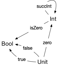
 .
. to
to  as:
as:  – that is, as exponentiation of the range of the produced functions.
 .
. , which we’ll call eval.
 and an element of
  which have the necessary product with
  is an object where the following product and arrow exist:
 to an object
  if the following conditions hold in the base category:
: X \rightarrow Y") in the base category.
in the base category.\times id_A: X\times A \rightarrow Y\times A")
\times id_A=\text{eval}_y y")
 .
. .
. which converts a value of
 \times\text{id}_A: X\times A \rightarrow Y\times A") , which given a pair
, which given a pair  \in X\times A") transforms it into a pair
transforms it into a pair  \in Y\times A") , where evaluating
, where evaluating =\text{eval}_y(\text{curry}(x, a))") . In other words, if we restrict the inputs to
. In other words, if we restrict the inputs to  might have a larger domain than the range of
  , and one from
  . Since the two arrows are deeply related (they’re one arrow in the category of potential exponentials), we’ll call them
 ") and
and \times id_A") . (Note that we’re not really taking the product of an arrow here: we haven’t talked about anything like taking products of arrows! All we’re doing is giving the arrow a name that helps us understand it. The name makes it clear that we’re not touching the right-hand component of the product.)
. (Note that we’re not really taking the product of an arrow here: we haven’t talked about anything like taking products of arrows! All we’re doing is giving the arrow a name that helps us understand it. The name makes it clear that we’re not touching the right-hand component of the product.) . Since
  represents the application of one of those functions to a value of type
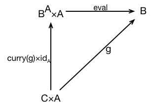
 , there is a unique function (arrow)
  to exist,
  , then we’ll say that
 ") , there exists a product object
, there exists a product object  , we say that the category has products.
 -calculus; and
 ") , where:
, where: is a collection of objects. We don’t actually care what the objects are – the only thing we can do in category theory is look at how the objects related through arrows that connect them. For a category
  is a collection of arrows, often called morphisms. Each element of
  that goes from
  to
to  , we’ll often write it as
  . For a category
  is a composition operator. For every pair of arrows
  , there must be an arrow
  called the compositions of
  .
. ") , there must be an arrow from
, there must be an arrow from  to
to  . For any arrow
  ; and for any arrow
  . That’s just a formal way of saying that composing an identity arrow with any other arrow results in the the other arrow.
 = (h\circ g)\circ f") .
.
 – because
 )") . You can read
. You can read =x^2") . That’s obviously a function from to Int to Int. Since Int is a set, it’s also an object in the category Set, and so
. That’s obviously a function from to Int to Int. Since Int is a set, it’s also an object in the category Set, and so  . .But there’s also a the set Int+, which represents the set of non-negative real numbers.
  is partially ordered if it has a partial less-than-or-equal relation,
  . This relation doesn’t need to be total – some values are less than or equal to other values; and some values can’t be compared.
 is order-preserving if and only if for all values
  , if
, if  in
in \le f(y)") in
in  is less than
  , then
 ") must be less than
must be less than ") .
. commutes if, for any two objects
 ") is the set of all paths in the diagram between
is the set of all paths in the diagram between ,: \circ(p_i) = \circ(p_j)") .
. and
and  . If this diagram commutes, it means that following
  from
from  .
.") then
then ") .
. and
and  . These arrows are objects in
  } There is an arrow from
  in
in ") if there is a pair of arrows
if there is a pair of arrows ") such that the following diagram commutes:
such that the following diagram commutes: .
.  into an arrow from
  .
. in category C is monic if for any pair of arrows
  and
and  in C,
in C,  implies that
  . (So a monic arrow discriminates arrows to its domain – every arrow to its domain from a given source will be mapped to a different codomain when left-composed with the monic.)
 in category C is epic if for any pair of arrows
  and
and  in C,
in C,  implies that
  can map onto
  in the same way as
  where
where  is epic, and where
  , and
, and  .
.") , there’s exactly one arrow
, there’s exactly one arrow ") . Similarly, a terminal object
. Similarly, a terminal object  in a category
  is an object where for every object
 ") .
. . How can that be? If
  , then from any other set
  is the constant function
  = t") . If
. If  is an element of a set
  to
to  to
to  .
. : a \in A, b \in B}.")
 , and each unique value
  , there’s a unique value
  \in A \times B") .
.") ? Mathematicians have come up with a lot of different ways of constructing ordered pairs. But we want to create a general model of an ordered pair, so we don’t want to limit ourselves to any specific construction: we want to capture the key property of what the ordered pair means.
? Mathematicians have come up with a lot of different ways of constructing ordered pairs. But we want to create a general model of an ordered pair, so we don’t want to limit ourselves to any specific construction: we want to capture the key property of what the ordered pair means. \in A\times B") , then
, then  = a") (where
(where  = b") (where
(where  is the name of the right projection).
 . This object has two special arrows,
  and
and  , that represent projections from
 ") . I can easily define a left project from
. I can easily define a left project from ") to
to  . It’s close, but it’s got extra noise attached, in the form of that third element
  from
from 

 and
and  , there is a unique arrow
 :C \rightarrow (A\times B)") for which the diagram to the right commutes.
for which the diagram to the right commutes. by an abelian group
  consists of a group
  together with an inclusion of
  as a normal subgroup and a surjective homomorphism
  that displays
  .
.") , where:
, where: is a set of values;
 is a total binary operator where:
 .
. * x = v * (w * x)")
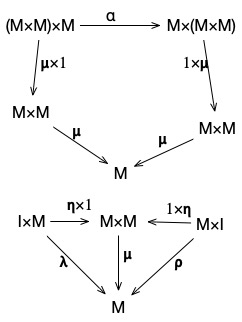
 is an arrow from
  , which we’ll call a multiplication operator.
 is an arrow from
  , called unit.
 is an arrow from
 \times M \rightarrow M \times (M\times M)") which represents the associativity property of the monoid.
which represents the associativity property of the monoid. ), and
 ") .
. \times M") composes with multiplication to be
composes with multiplication to be  .
.") .
.![A[\Gamma]](http://l.wordpress.com/latex.php?latex=A%5B%5CGamma%5D&bg=FFFFFF&fg=000000&s=0 "A[\Gamma]") , where A is a statement, and B is a set of assumptions. For example,
, where A is a statement, and B is a set of assumptions. For example, ![F(a) [a \in A, \Delta]](http://l.wordpress.com/latex.php?latex=F%28a%29%20%5Ba%20%5Cin%20A%2C%20%5CDelta%5D&bg=FFFFFF&fg=000000&s=0 "F(a) [a \in A, \Delta]") means that
means that ") is true, provided we’re in a context that includes
is true, provided we’re in a context that includes ![\frac{A \,\text{type}}{a \in A \,[a \in A]}](http://l.wordpress.com/latex.php?latex=%5Cfrac%7BA%20%5C%2C%5Ctext%7Btype%7D%7D%7Ba%20%5Cin%20A%20%5C%2C%5Ba%20%5Cin%20A%5D%7D&bg=FFFFFF&fg=000000&s=0 "\frac{A \,\text{type}}{a \in A \,[a \in A]}")
 is saying that
 ![\frac{a \in A \, []}{A \, \text{true}}](http://l.wordpress.com/latex.php?latex=%20%5Cfrac%7Ba%20%5Cin%20A%20%5C%2C%20%5B%5D%7D%7BA%20%5C%2C%20%5Ctext%7Btrue%7D%7D&bg=FFFFFF&fg=000000&s=0 "\frac{a \in A \, []}{A \, \text{true}}")


 in type
 ![C(x) \, \text{type} [x \in A]](http://l.wordpress.com/latex.php?latex=C%28x%29%20%5C%2C%20%5Ctext%7Btype%7D%20%5Bx%20%5Cin%20A%5D&bg=FFFFFF&fg=000000&s=0 "C(x) \, \text{type} [x \in A]") , which says that applying
, which says that applying ![\frac{C(x) \, \text{type} [x \in A] \quad a \in A}{C(a) \, \text{type}}](http://l.wordpress.com/latex.php?latex=%20%5Cfrac%7BC%28x%29%20%5C%2C%20%5Ctext%7Btype%7D%20%5Bx%20%5Cin%20A%5D%20%5Cquad%20a%20%5Cin%20A%7D%7BC%28a%29%20%5C%2C%20%5Ctext%7Btype%7D%7D&bg=FFFFFF&fg=000000&s=0 "\frac{C(x) \, \text{type} [x \in A] \quad a \in A}{C(a) \, \text{type}}")
") will be a type. In logical terms, it’s pretty straightforward; in programming terms it’s even clearer: if
will be a type. In logical terms, it’s pretty straightforward; in programming terms it’s even clearer: if ![\frac{C(x) \, \text{type}[x \in A] \quad a = b \in A}{C(a) = C(b)}](http://l.wordpress.com/latex.php?latex=%20%5Cfrac%7BC%28x%29%20%5C%2C%20%5Ctext%7Btype%7D%5Bx%20%5Cin%20A%5D%20%5Cquad%20a%20%3D%20b%20%5Cin%20A%7D%7BC%28a%29%20%3D%20C%28b%29%7D&bg=FFFFFF&fg=000000&s=0 "\frac{C(x) \, \text{type}[x \in A] \quad a = b \in A}{C(a) = C(b)}")
") isn’t quite a function. It’s a logical stamement which includes the symbol
isn’t quite a function. It’s a logical stamement which includes the symbol ![\frac{c(x) \in C(x) [x \in A] \quad a \in A}{c(a) \in C(A)}](http://l.wordpress.com/latex.php?latex=%20%5Cfrac%7Bc%28x%29%20%5Cin%20C%28x%29%20%5Bx%20%5Cin%20A%5D%20%5Cquad%20a%20%5Cin%20A%7D%7Bc%28a%29%20%5Cin%20C%28A%29%7D&bg=FFFFFF&fg=000000&s=0 "\frac{c(x) \in C(x) [x \in A] \quad a \in A}{c(a) \in C(A)}")
") is a proof-element: it’s an instance of
is a proof-element: it’s an instance of ") is a type, and we can see
is a type, and we can see  as a computation which, given an element of
 ") is an instance of type
is an instance of type ![\frac{c(x) \in C(x) [x \in A] \quad a = b}{c(a)=c(b)\in C(a)}](http://l.wordpress.com/latex.php?latex=%5Cfrac%7Bc%28x%29%20%5Cin%20C%28x%29%20%5Bx%20%5Cin%20A%5D%20%5Cquad%20a%20%3D%20b%7D%7Bc%28a%29%3Dc%28b%29%5Cin%20C%28a%29%7D&bg=FFFFFF&fg=000000&s=0 "\frac{c(x) \in C(x) [x \in A] \quad a = b}{c(a)=c(b)\in C(a)}")