With COVID running rampant throughout the US, I’ve seen a bunch of discussions about herd immunity, and questions about what it means. There’s a simple mathematical concept behind it, so I decided to spend a bit of time explaining.
The basic concept is pretty simple. Let’s put together a simple model of an infectious disease. This will be an extremely simple model – we won’t consider things like variable infectivity, population age distributions, population density – we’re just building a simple model to illustrate the point.
To start, we need to model the infectivity of the disease. This is typically done using the name . is the average number of susceptible people that will be infected by each person with the disease.
is the purest measure of infectivity – it’s the infectivity of the disease in ideal circumstances. In practice, we look for a value , which is the actual infectivity. includes the effects of social behaviors, population density, etc.
The state of an infectious disease is based on the expected number of new infections that will be produced by each infected individual. We compute that by using a number S, which is the proportion of the population that is susceptible to the disease.
If R S < 1, then the disease dies out without spreading throughout the population. More people can get sick, but each wave of infection will be smaller than the last.
If R S = 1, then the disease is said to be endemic. It continues as a steady state in the population. It never spreads dramatically, but it never dies out, either.
If R S > 1, then the disease is pandemic. Each wave of infection spreads the disease to a larger subsequent wave. The higher the value of in a pandemic, the faster the disease will spread, and the more people will end up sick.
There are two keys to managing the spread of an infectious disease
Reduce the effective value of . The value of can be affected by various attributes of the population, including behavioral ones. In the case of COVID-19, an infected person wearing a mask will spread the disease to fewer others; and if other people are also wearing masks, then it will spread even less.
Reduce the value of . If there are fewer susceptible people in the population, then even with a high value of , the disease can’t spread as quickly.
The latter is the key concept behind herd immunity. If you can get the value of to be small enough, then you can get to the sub-endemic level – you can prevent the disease from spreading. You’re effectively denying the disease access to enough susceptible people to be able to spread.
Let’s look at a somewhat concrete example. The for measles is somewhere around 15, which is insanely infectious. If 50% of the population is susceptible, and no one is doing anything to avoid the infection, then each person infected with measles will infect 7 or 8 other people – and they’ll each infect 7 or 8 others – and so on, which means you’ll have epidemic spread.
Now, let’s say that we get 95% of the population vaccinated, and they’re immune to measles. Now . The disease isn’t able to spread. If you had an initial outbreak of 5 infected, then they’ll infect around 3 people, who’ll infect around 2 people, who’ll infect one person, and soon, there’s no more infections.
In this case, we say that the population has herd immunity to the measles. There aren’t enough susceptible people in the population to sustain the spread of the disease – so if the disease is introduced to the population, it will rapidly die out. Even if there are individuals who are still susceptible, they probably won’t get infected, because there aren’t enough other susceptible people to carry it to them.
There are very few diseases that are as infectious as measles. But even with a disease that is that infectious, you can get to herd immunity relatively easily with vaccination.
Without vaccination, it’s still possible to develop herd immunity. It’s just extremely painful. If you’re dealing with a disease that can kill, getting to herd immunity means letting the disease spread until enough people have gotten sick and recovered that the disease can’t spread any more. What that means is letting a huge number of people get sick and suffer – and let some portion of those people die.
Getting back to COVID-19: it’s got an that’s much lower. It’s somewhere between 1.4 and 2.5. Of those who get sick, even with good medical care, somewhere between 1 and 2% of the infected end up dying. Based on that , herd immunity for COVID-19 (the value of S required to make R*S<1) is somewhere around 50% of the population. Without a vaccine, that means that we’d need to have 150 million people in the US get sick, and of those, around 2 million would die.
(UPDATE: Ok, so I blew it here. The papers that I found in a quick search appear to have a really bad estimate. The current CDC estimate of is around 5.7 – so the S needed for herd immunity is significantly higher – upward of 80%, and so the would the number of deaths.)
A strategy for dealing with an infection disease that accepts the needless death of 2 million people is not exactly a good strategy.
In my last post about category theory, I introduced the basic idea of typeclasses, and showed how to implement an algebraic monoid as a typeclass. Then we used that algebraic monoid as an example of how to think with arrows, and built it up into a sketch of category theory’s definition of a monoid. We ended with an ominous looking diagram that illustrated what a categorical monoid looks like.
In this post, we’re going to take a look at some of the formal definitions of the basic ideas of category theory. By the end of this lesson, you should be able to look at the categorical monoid, and understand what it means. But the focus of this post will be on understanding initial and terminal objects, and the role they play in defining abstractions in category theory. And in the next post, we’ll see how abstractions compose, which is where the value of category theory to programmers will really become apparrent.
Before I really get started: there’s a lot of terminology in category theory, and this post has a lot of definitions. Don’t worry: you don’t need to remember it all. You do need to understand the concepts behind it, but specifically remembering the difference between, say, and endomorphism, and epimorphism, and a monomorphism isn’t important: you can always look it up. (And I’ll put together a reference glossary to help make that easy.)
Defining Categories
A category is basically a directed graph – a bunch of dots connected by arrows, where the arrows have to satisfy a bunch of rules.
Formally, we can say that a category consists of a the parts: , where:
is a collection of objects. We don’t actually care what the objects are – the only thing we can do in category theory is look at how the objects related through arrows that connect them. For a category , we’ll often call this collection Obj(C).
is a collection of arrows, often called morphisms. Each element of starts at one object called its domain (often abbreviated dom), and ending at another object called its codomain (abbreviated cod). For an arrow that goes from to , we’ll often write it as . For a category , we’ll often call this set Mor(C) (for morphisms of C).
is a composition operator. For every pair of arrows , and , there must be an arrow called the compositions of and .
To be a category, these must satisfy the following rules:
Identity: For every object , there must be an arrow from to , called the identity of . We’ll often write it as . For any arrow ; and for any arrow . That’s just a formal way of saying that composing an identity arrow with any other arrow results in the the other arrow.
Associativity: For any set of arrows .
When talking about category theory, people often say that an arrow is a structure preserving mapping between objects. We’ll see what that means in slightly more detail with some examples.
A thing that I keep getting confused by involves ordering. Let’s look at a quick little diagram for a moment. The path from X to Z is – because comes after , which (at least to me) looks backwards. When you write it in terms of function application, it’s . You can read as g after f, because the arrow comes after the arrow in the diagram; and if you think of arrows as functions, then it’s the order of function application.
Example: The category Set
The most familiar example of a category (and one which is pretty canonical in category theory texts) is the category Set, where the objects are sets, the arrows between them are total functions, and the composition operator is function composition.
That might seem pretty simple, but there’s an interesting wrinkle to Set.
Suppose, for example, that we look at the function . That’s obviously a function from to Int to Int. Since Int is a set, it’s also an object in the category Set, and so is obviously an arrow from . .But there’s also a the set Int+, which represents the set of non-negative real numbers. is also a function from Int+ to Int+. So which arrow represents the function?
The answer is both – and many more. (It’s also a function from the reals to complex numbers, because every real number is also a complex number.) And so on. A function isn’t quite an arrow: an arrow is a categorical concept of some kind of mapping between two objects. In many ways, you can think of an arrow as something almost like a function with an associated type declaration: you can write many type declarations for a given function; any valid function with a type declaration that is an arrow in Set.
We’ll be looking at Set a lot. It’s a category where we have a lot of intuition, so using it as an example to demonstrate category concepts will be useful.
Example: The category Poset
Poset is the category of all partially ordered sets. The arrows between objects in posets are order-preserving functions between partially ordered sets. This category is an example of what we mean by structure-preserving mappings: the composition operator must preserve the ordering property.
For that to make sense, we need to remember what partially ordered set is, and what it means to be an order preserving function.
A set is partially ordered if it has a partial less-than-or-equal relation, . This relation doesn’t need to be total – some values are less than or equal to other values; and some values can’t be compared.
A function between two partially ordered sets is order-preserving if and only if for all values , if in , then in .
The key feature of an object in Poset is that is possesses a partial ordering. So arrows in the category must preserve that ordering: if is less than , then must be less than .
That’s a typical example of what we mean by arrows as structure preserving: the objects of a category have some underlying structural property – and to be an arrow in the category, that structure must be preserved across arrows and arrow composition.
Commuting Diagrams
One of the main terms that you’ll hear about category diagrams is about whether or not the diagram commutes. This, in turn, is based on arrow chasing.
An arrow chase is a path through the diagram formed by chaining arrows together by composing them – an arrow chase is basically discovering an arrow from one object to another by looking at the composition of other arrows in the category.
We say that a diagram commutes if, for any two objects and in the diagram, every pair of paths between and compose to the same arrow. Another way of saying that is that if is the set of all paths in the diagram between and , .
For example: In this diagram, we can see two paths: and . If this diagram commutes, it means that following from to and from to must be the same thing as following from to and from to . It doesn’t say that and are the same thing – an arrow chase doesn’t tell us anything about single arrows; it just tells us about how they compose. So what we know if this diagram commutes is that .
Diagrams and Meta-level reasoning: an example
Let’s look at a pretty tricky example. We’ll take our time, because this is subtle, but it’s also pretty typical of how we do things in category theory. One of the key concepts of category theory is building a category, and then using the arrows in that category, create a new category that allows us to do meta-level reasoning.
We’ve seen that there’s a category of sets, called Set.
We can construct a category based on the arrows of Set, called Set→. In this category, each of the arrows in Set is an object. So, more formally, if then .
The arrows of this new category are where it gets tricky. Suppose we have two arrows in Set, and . These arrows are objects in } There is an arrow from to in if there is a pair of arrows and in such that the following diagram commutes:
commuting diagram for arrows in set-arrow
The diagram is relatively easy to read and understand; explaining it in works is more complicated:
an arrow in our category of Set-arrows is a mapping from one Set-arrow to another Set-arrow .
That mapping exists when there are two arrows and in where:
is an arrow from the domain of to the domain of ;
is an arrow from the codomain of to the codomain of ; and
.
Another way of saying that is that there’s an arrow means that there’s a structure-preserving way of transforming any arrow from into an arrow from .
Why should we care about that? Well, for now, it’s just a way of demonstrating that a diagram can be a lot easier to read than a wall of text. But this kind of categorical mapping will become important later.
Categorizing Things
As I said earlier, category theory tends to have a lot of jargon. Everything we do in category theory involves reasoning about arrows, so there are many terms that describe arrows with particular properties. We’ll look at the most basic categories now, and we’ll encounter more in later lessons.
Monics, Epics, and Isos
The easiest way to think about all of these categories is by analogy with functions in traditional set-based mathematics. Functions and their properties are really important, so we define special kinds of functions with interesting categories. We have injections (functions from A to B where every element of A is mapped onto a unique element of B), surjections (functions from A to B where each element of B is mapped onto by an element of A), and isomorphisms.
In categories, we define similar categories: monomorphisms (monics), epimorphisms (epics), and isomorphisms (isos).
An arrow in category C is monic if for any pair of arrows and in C, implies that . (So a monic arrow discriminates arrows to its domain – every arrow to its domain from a given source will be mapped to a different codomain when left-composed with the monic.)
An epic is almost the same, except that it discriminates with right-composition: An arrow in category C is epic if for any pair of arrows and in C, implies that . (So in the same way that a monic arrow discriminations arrows to its domain, an epic arrow discriminates arrows from its codomain.)
These definitions sound really confusing. But if you think back to sets, you can twist them into making sense. A monic arrow describes an injection in set theory: that is, a function maps every element of onto a unique element of . So if you have some functions and that maps from some set onto , then the only way that can map onto in the same way as is if and map onto in exactly the same way.
The same basic argument (reversed a bit) can show that an epic arrow is a surjective function in Set.
An isomorphism is a pair of arrows and where is monic and is epic, and where , and .
We say that the objects and are isomorphic if there’s an isomorphism between them.
Initial and Terminal Objects
Another kind of categorization that we look at is talking about special objects in the category. Categorical thinking is all about arrows – so even when we’re looking at special objects, what make them special are the arrows that they’re related to.
An initial object 0 in a category is an object where for every object , there’s exactly one arrow . Similarly, a terminal object in a category is an object where for every object , there is exactly one arrow .
For example, in the category Set, the empty set is an initial object, and singleton sets are terminal objects.
A brief interlude:
What’s the point?In this lesson, we’ve spent a lot of time on formalisms and definitions of abstract concepts: isos, monos, epics, terminals. And after this pause, we’re going to spend a bunch of time on building some complicated constructions using arrows. What’s the point of all of this? What does any of these mean?
Underlying all of these abstractions, category theory is really about thinking in arrows. It’s about building structures with arrows. Those arrows can represent import properties of the objects that they connect, but they do it in a way that allows us to understand them solely in terms of the ways that they connect, without knowing what the objects connected by the arrows actually do.
In practice, the objects that we connect by arrows are usually some kind of aggregate: sets, types, spaces, topologies; and the arrows represent some kind of mapping – a function, or a transformation of some kind. We’re reasoning about these aggregates by reasoning about how mappings between the aggregates behave.
But if the objects represent some abstract concept of collections or aggregates, and we’re trying to reason about them, sometimes we need to be able to reason about what’s inside of them. Thinking in arrows, the only way to really be able to reason about a concept like membership, the only way we can look inside the structure of an object, is by finding special arrows.
The point of the definitions we just looked at is to give us an arrow-based way of peering inside of the objects in a category. These tools give us the ability to create constructions that let us take the concept of something like membership in a set, and abstract it into an arrow-based structure.
Reasoning in arrows, a terminal object is an object in a category that captures a concept of a single object. It’s easiest to see this by thinking about sets as an example. What does it mean if an object, T, is terminal in the category of sets?
It means that for every set , there’s exactly one function from to . How can that be? If is a set containing exactly one value , then from any other set , the only function from is the constant function . If had more than one value in it, then it would be possible to have more than one arrow from to – because it would be possible to define different functions from to .
By showing that there’s only one arrow from any object in the category of sets to T, we’re showing that can’t possibly have more than one object inside of it.
Knowing that, we can use the concept of a terminal object to create a category-theoretic generalization of the concept of set membership. If is an element of a set , then that set membership can be represented by the fact that there is an arrow from the terminal object to . In general, for any object in a category, if there is an arrow from a terminal object to , then in some sense, .
Constructions
We’re finally getting close to the real point of category theory. Category theory is built on a highly abstracted notion of functions – arrows – and then using those arrows for reasoning. But reasoning about individual arrows only gets you so far: things start becoming interesting when you start constructing things using arrows. In lesson one, we saw a glimpse of how you could construct a very generalized notion of monoid in categories – this is the first big step towards understanding that.
Products
Constructions are ways of building things in categories. In general, the way that we work with constructions is by defining some idea using a categorical structure – and then abstracting that into something called a universal construction. A universal construction defines a new category whose objects are instances of the categorical structure; and we can understand the universal construction best by looking at the terminal objects in the universal construction – which we can understand as being the atomic objects in its category.
When we’re working with sets, we know that there’s a set-product called the cartesian product. Given two sets, A and B, the product
The basic concept of a product is really useful. We’ll eventually build up to something called a closed cartesian category that uses the categorical product, and which allows us to define the basis of lambda calculus in category theory.
As usual, we want to take the basic concept of a cartesian product, and capture it in terms of arrows. So let’s look back at what a cartesian product is, and see how we can turn that into arrow-based thinking.
The simple version is what we wrote above: given two sets A and B, the cartesian product maps them into a new set which consists of pairs of values in the old set. What does that mean in terms of arrows? We can start by just slightly restating the definition we gave above: For each unique value , and each unique value , there’s a unique value .
But what do we actually mean by ? Mathematicians have come up with a lot of different ways of constructing ordered pairs. But we want to create a general model of an ordered pair, so we don’t want to limit ourselves to any specific construction: we want to capture the key property of what the ordered pair means.
It doesn’t matter which one we use: what matters is that there’s a key underlying property of the product: there are two functions and, called projection functions, which map elements of the product back to the elements of A and B. If , then (where is the name of the left projection), and (where is the name of the right projection).
That’s going to be the key to the categorical product: it’s going to be defined primarily by the projection functions. We know that the only way we can talk about things in category theory is to use arrows. The thing that matters about a product is that it’s an object with projections to its two parts. We can describe that, in category theory, as something that we’ll call a wedge:
The wedge: a candidate for a product.
A wedge is basically an object, like the one in the diagram to the right, which we’ll call . This object has two special arrows, and , that represent projections from to its components in and .
Now we get to the tricky part. The concept of a wedge captures the structure of what we mean by a product. But given two objects A and B, there isn’t just one wedge! In a category like Set, there are many different ways of creating objects with projections. Which object is the correct one to use for the product?
For example, I can have the set of triples . I can easily define a left project from to , and a right projection from to . But clearly is not what we mean by the product of . It’s close, but it’s got extra noise attached, in the form of that third element .
If, for two objects and , there are many wedges with left and right projections, which one is the real product?
Just a little while ago, we talked about initial and terminal objects. A terminal object can be understood as being a rough analog to a membership relation. We’re going to use that. We can create a category of wedges , where there is an arrow from to when the diagram below commutes in our original category:
The ideal product: the terminal in the category of wedges.
In the category of wedges, what that means is that Y is at least as strict of a wedge than X; X has some amount of noise in it (noise in the sense of the C element of the triple from the example above), and Y cannot have any more noise than that. The true categorical product will be the wedge with no excess noise: an wedge which has an arrow from every other wedge in the category of wedges. What’s an object with an edge from every other object? It’s the terminal object. The categorical product is the terminal wedge: the unique (up to isomorphism) object which is stricter than any other wedge. Another way of saying that, using categorical terminology, is that there is a universal property of products: products have left and right projections. The categorical product is the exemplar of that property: it is the unique object which has exactly the property that we’re looking at, without any extraneous noise. Any property that this universal object has will be shared by every other product-like object.
This diagram should look familiar: it’s the same thing as the diagram for defining arrows in the category of wedges. It’s the universal diagram: you can substitute any wedge in for C, along with its project arrows (f, g).
The categorical product.
We can pull that definition back to our original category, and define the product without the category of wedges. So given two objects, A and B, in a category, the categorical product is defined as an object which we’ll call along with two arrows and , which have the property that for any object which has arrows and , there is a unique arrow for which the diagram to the right commutes.
On its own, if we’re looking specifically at sets, this is just a complicated way of defining the cartesian product of two values. It doesn’t really tell us much of anything new. What makes this interesting is that it isn’t limited to the cartesian product of two sets: it’s a general concept that takes what we understand about simple sets, and expands it to define a product of any two things in categories. The set-theoretic version only works for sets: this one works for numbers, posets, topologies, or anything else.
In terms of programming, products are pretty familiar to people who write functional programs: a product is a tuple. And the definition of a tuple in a functional language is pretty much exactly what we just described as the categorical product, tweaked to make it slightly easier to use.
For example, let’s look at the product type in Scala.
trait Product extends Any with Equals {
  def productElement(n: Int): Any
  def productArity: Int
...
}
The product object intrinsically wraps projections into a single function which takes a parameter and returns the result of applying the projection. It could have been implemented more categorically as:
trait CatProduct extends Any with Equals {
  def projection(n: Int): () => Any
  ...
}
Implemented the latter way, to extract an element from a product, you’d have to write prod.projection(i)() which is more cumbersome, but does the same thing.
More, if you look at this, and think of how you’d use the product trait, you can see how it relates to the idea of terminal objects. There are many different concrete types that you could use to implement this trait. All of them define more information about the type. But every implementation that includes the concept of product can implement the Product trait. This is exactly the relationship we discussed when we used terminal objects to derive the ideal product: there are many abstractions that include the concept of the product; the categorical product is the one that abstracts over all of them.
The categorical product, as an abstraction, may not seem terribly profound. But as we’ll see in a the next post, in category theory, we can compose abstractions – and by using composition to in a compositional way, we’ll be able to define an abstraction of exponentiation, which generalizes the programming language concept of currying.
One thing that I keep bumping up against as an engineer who loves functional a programming is category theory. It often seems like there are two kinds of functional programmers: people who came into functional programming via engineering, and people who came into functional programming via math. The problem is that a lot of the really interesting work in languages and libraries for functional programming are being built from the mathematical side, but for people on the engineering side, it’s impenetrable: it’s like it’s written in a whole different language, and even basic discussions about programming go off the rails, because the basic abstractions don’t make any sense if you don’t know category theory.
But how do you learn category theory? It seems impenetrable to mere humans. For example, one of the textbooks on category theory that several people told me was the most approachable starts chapter one with the line:
A group extension of an abelian group by an abelian group consists of a group together with an inclusion of as a normal subgroup and a surjective homomorphism that displays as the quotient group .
If you’re not a professional mathematician, then that is pure gobbledigook. But that seems to be typical of how initiates of category theory talk about it. But the basic concepts, while abstract, really aren’t all that tricky. In many ways, it feels a lot like set theory: there’s a simple conceptual framework, on which you can build extremely complicated formalisms. The difference is that while many people have spent years figuring out how to make the basics of set theory accessible to lay-people, but that effort hasn’t been applied to set theory.
What’s the point?
Ok, so why should you care about category theory?
Category theory is a different way of thinking, and it’s a language for talking about abstractions. The heart of engineering is abstraction. We take problems, and turn them into abstract structures. We look at the structures we create, and recognize commonalities between those structures, and then we create new abstractions based on the commonalities. The hardest part of designing a good library is identifying the right abstractions.
Category theory is a tool for talking about structures, which is particularly well suited to thinking about software. In category theory, we think in terms of arrows, where arrows are mappings between objects. We’ll see what that means in detail later, but the gist of it is that one example of arrows mapping between objects is functions mapping between data types in a computer program.
Category theory is built on thinking with orrows, and building structures using arrows. It’s about looking at mathematical constructions built with arrows, and in those structures, figuring out what the fundamental parts are. When we abstract enough, we can start to see that things that look very different are really just different realizations of the same underlying structure. Category theory gives us a language and a set of tools for doing that kind of abstraction – and then we can take the abstract structures that we identify, and turn them into code – into very generic libraries that express deep, fundamental structure.
Start with an Example: Monoids
Monoids in Code
We’ll get started by looking at a simple mathematical structure called a monoid, and how we can implement it in code; and then, we’ll move on to take an informal look at how it works in terms of categories.
Most of the categorical abstractions in Scala are implemented using something called a typeclass, so we’ll start by looking at typeclasses. Typeclasses aren’t a category theoretical notion, but they make it much, much easier to build categorical structures. And they do give us a bit of categorical flavor: a typeclass defines a kind of metatype – that is, a type of type – and we’ll see, that kind of self-reflective abstraction is a key part of category theory.
The easiest way to think about typeclasses is that they’re a kind of metatype – literally, as the name suggests, they define classes where the elements of those classes are types. So a typeclass provides an interface that a type must provide in order to be an instance of the metatype. Just like you can implement an interface in a type by providing implementations of its methods, you can implement a typeclass by providing implementations of its operations.
In Scala, you implement the operations of a typeclasses using a language construct called an implicit parameter. The implicit parameter attaches the typeclass operations to a meta-object that can be passed around the program invisibly, providing the typeclass’s operations.
Let’s take a look at an example. An operation that comes up very frequently in any kind of data processing code is reduction: taking a collection of values of some type, and combining them into a single value. Taking the sum of a list of integers, the product of an array of floats, and the concatenation of a list of strings are all examples of reduction. Under the covers, these are all similar: they’re taking an ordered group of values, and performing an operation on them. Let’s look at a couple of examples of this:
When you look at the code, they look very similar. They’re both just instantiations of the same structural pattern:
def reduceX(xes: List[X]): X =
    xes.foldRight(xIdentity)((a, b) => Xcombiner(a, b))
The types are different; the actual operation used to combine the values is different; the base value in the code is different. But they’re both built on the same pattern:
There’s a type of values we want to combine: Float or String. Everything we care about in reduction is a connected with this type.
There’s a collection of values that we want to combine, from left to right. In one case, that’s a List[Float], and in the other, it’s a Seq[String]. The type doesn’t matter, as long as we can iterate over it.
There’s an identity value that we can use as a starting point for building the result; 0 for the floats, and "" (the empty string) for the strings.
There’s an operation to combine two values: + for the floats, and concat for the strings.
We can capture that concept by writing an interface (a trait, in Scala terms) that captures it; that interface is called a typeclass. It happens that this concept of reducible values is called a monoid in abstract algebra, so that’s the name we’ll use.
trait Monoid[A]  {
    def empty: A
    def combine(x: A, y: A): A
}
We can read that as saying “A is a monoid if there are implementations of empty and combine that meet these constraints”. Given the declaration of the typeclass, we can implement it as an object which provides those operations for a particular type:
FloatAdditionMonoid implements the typeclass Monoid for the type Float. And since we can write an implementation of Monoid for Float or String, we can say that the types Float and String are instances of the typeclass Monoid.
Using our implementation of Monoid, we can write a single, generic reduction operator now:
def reduce[A](values: Seq[A], monoid: Monoid[A]): A =
   values.foldRight(monoid.empty)(monoid.combine)
And we can do a bit better than that! We can set up an implicit, so that we don’t need to pass the monoid implementation around. In Scala, an implicit is a kind of dynamically scoped value. For a given type, there can be one implicit value of that type in effect at any point in the code. If a function takes an implicit parameter of that type, then the nearest definition in the execution stack will automatically be inserted if the parameter isn’t passed explicitly.
def reduce[A](values: Seq[A])(implicit A: Monoid[A]): A =
   list.foldRight(A.empty)(A.combine)
And as long as there’s a definition of the Monoid for a type A in scope, we can can use that now by just writing:
implicit object FloatAdditionMonoid extends Monoid[Float] {
    def empty: Float = 0.0
    def combine(x: Float, y: Float): Float = x + y
}

val floats: List[Float] = ...
val result = reduce(floats)
Now, anywhere that the FloatAdditionMonoid declaration is imported, you can call reduce on any sequence of floats, and the implicit value will automatically be inserted.
Using this idea of a monoid, we’ve captured the concept of reduction in a common abstraction. Our notion of reduction doesn’t care about whether we’re reducing strings by concatenation, integers by addition, floats by multiplication, sets by union. Those are all valid uses of the concept of a monoid, and they’re all easy to implement using the monoid typeclass. The concept of monoid isn’t a difficult one, but at the same time, it’s not necessarily something that most of us would have thought about as an abstraction.
We’ve got a typeclass for a monoid; now, we’ll try to connect it into category theory. It’s a bit tricky, so we won’t cover it all at once. We’ll look at it a little bit now, and we’ll come back to it in a later lesson, after we’ve absorbed a bit more.
From Sets to Arrows
For most of us, if we’ve heard of monoids, we’ve heard of them in terms of set theory and abstract algebra. So in that domain, what’s a monoid?
A monoid is a triple , where:
is a set of values;
is a value in ;
is a total binary operator where:
is an identity of : For any value .
is associative: for any values
That’s all just a formal way of saying that a monoid is a set with a binary associative operator and an identity value. The set of integers can form a monoid with addition as the operator, and 0 as identity. Real numbers can be a monoid with multiplication and 1. Strings can be a monoid with concatenation as the operator, and empty string as identity.
But we can look at it in a different way, too, by thinking entirely in terms of function.
Let’s forget about the numbers as individual values, and instead, let’s think about them in functional terms. Every number is a function which adds itself to its parameter. So “2” isn’t a number, it’s a function which adds two to anything.
How can we tell that 2 is a function which adds two to things?
If we compose it with 3 (the function that adds three to things), we get 5 (the function that adds five to things). And how do we know that? Because it’s the same thing that we get if we compose 3 with 1, and then compose the result of that with 1 again. 3+1+1=5, and 3+2=5. We can also tell that it’s 2, because if we just take 1, and compose it with itself, what we’ll get back is the object that we call 2.
In this scheme, all of the numbers are related not by arithmetic, not by an underlying concept of quantity or cardinality or ordinality, but only by how they compose with each other. We can’t see anything else – all we have are these functions. But we can recognize that they are the natural numbers that we’re familiar with.
Looking at it this way, we can think of the world of natural numbers as a single point, which represents the set of all natural numbers. And around that point, we’ve got lots and lots of arrows, each of which goes from that point back to itself. Each of those arrows represents one number. The way we tell them apart is by understanding which arrow we get back when we compose them. Take any arrow from that point back to that point, and compose it with the arrow 0, and what do you get? The arrow you started with. Take any arrow that you want, and compose it with 2. What do you get? You get the same thing that you’d get if you composed it with 1, and then composed it with one again.
That dot, with those arrows, is a category.
What kind of advantage do we get in going from the algebraic notion of a set with a binary operation, to the categorical notion of an object with a bunch of composable arrows? It allows to understand a monoid purely as a structure, without having the think about what the objects are, or what the operator means.
Now, let’s jump back to our monoid typeclass for a moment.
trait Monoid[A]  {
    def empty: A
    def combine(x: A, y: A): A
}
We can understand this as being a programmable interface for the categorical object that we just described. All we need to do is read “:” as “is an arrow in”: It says that A is a monoid if:
It has an element called empty which is an arrow in A.
It has an operation called combine which, given any two arrows in A, composes them into a new arrow in A.
There are, of course, other conditions – combine needs to be associative, and empty needs to behave as the identity value. But just like when we write an interface for, say, a binary search tree, the interface only defines the structure not the ordering condition, the typeclass defines the functional structure of the categorical object, not the logical conditions.
This is what categories are really all about: tearing things down to a simple core, where everything is expressed in terms of arrows. It’s almost reasoning in functions, except that it’s even more abstract than that: the arrows don’t need to be functions – they just need to be composable mappings from things to things.
Deeper Into Arrows
We can abstract a bit more, and look at the entire construction, including the identity and associativity constraints entirely in terms of arrows. To really understand this, we’ll need to spend some time diving deeper into the actual theory of categories, but as a preview, we can describe a monoid with the following pair of diagrams (copied from wikipedia):
In these diagrams, any two paths between the same start and end-nodes are equivalent (up to isomorphism). When you understand how to read this diagrams, these really do define everything that we care about for monoids.
For now, we’ll just run through and name the parts – and then later, in another lesson, we’ll come back, and we’ll look at this in more detail.
is an arrow from , which we’ll call a multiplication operator.
is an arrow from , called unit.
is an arrow from which represents the associativity property of the monoid.
is a morphism which represents the left identity property of the monoid (that is, ), and is a morphism representing the right identity property .
This diagram, using these arrows, is a way of representing all of the key properties of a monoid via nothing but arrows and composition. It says, among other things, that:
composes with multiplication to be .
That is, applying multiplication to evaluates to (M \times M).
composed with associativity can become .
So it’s a monoid – but it’s a higher level monoid. In this, isn’t just an object in a category: it’s an entire category. These arrows are arrows between categories in a category of categories.
What we’ll see when we get deeper into category theory is how powerful this kind of abstraction can get. We’ll often see a sequence of abstractions, where we start with a simple concept (like monoid), and find a way to express it in terms of arrows between objects in a category. But then, we’ll lift it up, and look at how we can see in not just as a relation between objects in a category, but as a different kind of relation between categories, by constructing the same thing using a category of categories. And then we’ll abstract even further, and construct the same thing using mappings between categories of categories.
(You can find the next lesson <a href=”http://www.goodmath.org/blog/2019/02/20/category-theory-lesson-2-basics-of-categorical-abstraction/”>here</a>.)
It’s been quite a while since I did any meaningful writing on type theory. I spent a lot of time introducing the basic concepts, and trying to explain the intuition behind them. I also spent some time describing what I think of as the platform: stuff like arity theory, which we need for talking about type construction. But once we move beyond the basic concepts, I ran into a bit of a barrier – no so much in understanding type theory, but in finding ways of presenting it that will be approacha ble.
I’ve been struggling to figure out how to move forward in my exploration of type theory. The logical next step is working through the basics of intuitionistic logic with type theory semantics. The problem is, that’s pretty dry material. I’ve tried to put together a couple of approaches that skip over this, but it’s really necessary.
For someone like me, coming from a programming language background, type theory really hits its stride when we look at type systems and particularly type inference. But you can’t understand type inference without understanding the basic logic. In fact, you can’t describe the algorithm for type inference without referencing the basic inference rules of the underlying logic. Type inference is nothing but building type theoretic proofs based on a program.
So here we are: we need to spend some time looking at the basic logic of type theory. We’ve looked at the basic concepts that underlie the syntax and semantics, so what we need to do next is learn the basic rules that we use to build logical statements in the realm of type theory. (If you’re interested in more detail, this is material from chapter 5 of “Programming in Martin-Löof’s Type Theory”, which is the text I’m using to learn this material.)
Martin Löoff’s type theory is a standard intuitionistic predicate logic, so we’ll go through the rules using standard sequent notation. Each rule is a sequence which looks sort-of like a long fraction. The “numerator” section is a collection of things which we already know are true; the “denominator” is something that we can infer given those truths. Each statement has the form , where A is a statement, and B is a set of assumptions. For example, means that is true, provided we’re in a context that includes .
Personally, I find that this stuff feels very abstract until you take the logical statements, and interpret them in terms of programming. So throughout this post, I’ll do that for each of the rules.
With that introduction out of the way, let’s dive in to the first set of rules.
Simple Introductions
We’ll start off with a couple of really easy rules, which allow us to introduce a variable given a type, or a type given a variable.
Introducing Elements
This is an easy one. It says that if we know that A is a type, then we can introduce the statement that , and add that as an assumption in our context. What this means is also simple: since our definition of type says that it’s only a type if it has an element, then if we know that A is a type, we know that there must be an element of A, and so we can write statements using it.
If you think of this in programming terms, the statement is saying that is a type. To be a valid type, there must be at least one value that belongs to the type. So you’re allowed to introduce a variable that can be assigned a value of the type.
Introducing Propositions as Types
This is almost the mirror image of the previous. A type and a true proposition are the same thing in our type theory: a proposition is just a type, which is a set with at least one member. So if we know that there’s a member of the set A, then A is both a type and a true proposition.
Equality Rules
We start with the three basic rules of equality: equality is reflexive, symmetric, and transitive.
Reflexivity
If is an element of a type , then is equal to itself in type ; and if is a type, then is equal to itself.
The only confusing thing about this is just that when we talk about an object in a type, we make reference to the type that it’s a part of. This makes sense if you think in terms of programming: you need to declare the type of your variables. “3: Int” doesn’t necessarily mean the same object as “3: Real”; you need the type to disambiguate the statement. So within type theory, we always talk about values with reference to the type that they’re a part of.
Symmetry
No surprises here – standard symmetry.
Transitivity
Type Equality
These are pretty simple, and follow from the basic equality rules. If we know that is a member of the type , and we know that the type equals the type , then obviously is also a member of . Along the same lines, if we know that in type , and equals , then in the type .
Substitution Rules
We’ve got some basic rules about how to formulate some simple meaningful statements in the logic of our type theory. We still can’t do any interesting reasoning; we haven’t built up enough inference rules. In particular, we’ve only been looking at simple, atomic statements using parameterless predicates.
We can use those basic rules to start building upwards, to get to parametric statements, by using substitution rules that allow us to take a parametric statement and reason with it using the non-parametric rules we talked about above.
For example, a parametric statement can be something like , which says that applying to a value which is a member of type produces a value which is a type. We can use that to produce new inference rules like the ones below.
This says that if we know that given a of type , will produce a type; and we know that the value is of type , then will be a type. In logical terms, it’s pretty straightforward; in programming terms it’s even clearer: if is a function on type , and we pass it a value of type , it will produce a result. In other words, is defined for all values of type .
This is even simpler: if is a function on type , then given two values that are equal in type , will produce the same result for those values.
Of course, I’m lying a bit. In this stuff, isn’t really a function. It’s a logical statement; isn’t quite a function. It’s a logical stamement which includes the symbol ; when we say , what we mean is the logical statement , with the object substituted for the symbol . But I think the programming metaphors help clarify what it means.
Using those two, we can generate more:
This one becomes interesting. is a proposition which is parametric in . Then is a proof-element: it’s an instance of which proves that is a type, and we can see as a computation which, given an element of produces a instance of . Then what this judgement says is that given an instance of type , we know that is an instance of type . This will become very important later on, when we really get in to type inference and quantification and parametric types.
This is just a straightforward application of equality to proof objects.
There’s more of these kinds of rules, but I’m going to stop here. My goal isn’t to get you to know every single judgement in the intuitionistic logic of type theory, but to give you a sense of what they mean.
That brings us to the end of the basic inference rules. The next things we’ll need to cover are ways of constructing new types or types from existing ones. The two main tools for that are enumeration types (basically, types consisting of a group of ordered values), and cartesian products of multiple types. With those, we’ll be able to find ways of constructing most of the types we’ll want to use in programming languages.
There’s a lot of talk today about the recent discovery of a significant bug in the Intel CPUs that so many of us use every day. It’s an interesting problem, and understanding it requires knowing a little bit about how CPUs work, so I thought I’d take a shot at writing an explainer.
Let me start with a huge caveat: this involves a lot of details about how CPUs work, and in order to explain it, I’m going to simplify things to an almost ridiculous degree in order to try to come up with an explanation that’s comprehensible to a lay person. I’m never deliberately lying about how things work, but at times, I’m simplifying enough that it will be infuriating to an expert. I’m doing my best to explain my understanding of this problem in a way that most people will be able to understand, but I’m bound to oversimplify in some places, and get details wrong in others. I apologize in advance.
It’s also early days for this problem. Intel is still trying to keep the exact details of the bug quiet, to make it harder for dishonest people to exploit it. So I’m working from the information I’ve been able to gather about the issue so far. I’ll do my best to correct this post as new information comes out, but I can only do that when I’m not at work!
That said: what we know so far is that the Intel bug involves non-kernel code being able to access cached kernel memory through the use of something called speculative execution.
To an average person, that means about as much as a problem in the flux thruster atom pulsar electrical ventury space-time implosion field generator coil.
Let’s start with a quick overview of a modern CPU.
The CPU, in simple terms, the brain of a computer. It’s the component that actually does computations. It reads a sequence of instructions from memory, and then follows those instructions to perform some computation on some values, which are also stored in memory. This is a massive simplification, but basically, you can think of the CPU as a pile of hardware than runs a fixed program:
def simplified_cpu_main_loop():
  IP = 0
  while true:
     (op, in1, in2, out) = fetch(IP)
     val1 = fetch(in1)
     val2 = fetch(in2)
     result, IP = perform(op, in1, in2)
     store(result, out)
There’s a variable called the instruction pointer (abbreviated IP) built-in to the CPU that tells it where to fetch the next instruction from. Each time the clock ticks, the CPU fetches an instruction from the memory address stored in the instruction pointer, fetches the arguments to that instruction from cells in memory, performs the operation on those arguments, and then stores the result into another cell in the computer memory. Each individual operation produces both a result, and a new value for the instruction pointer. Most of the time, you just increment the instruction pointer to look at the next instruction, but for comparisons or branches, you can change it to something else.
What I described above is how older computers really worked. But as CPUs got faster, chipmaker ran into a huge problem: the CPU can perform its operations faster and faster every year. But retrieving a value from memory hasn’t gotten faster at the same rate as executing instructions. The exact numbers don’t matter, but to give you an idea, a modern CPU can execute an instruction in less than one nanosecond, but fetching a single value from memory takes more than 100 nanoseconds. In the scheme we described above, you need to fetch the instruction from memory (one fetch), and then fetch two parameters from memory (another two fetches), execute the instruction (1 nanosecond), and then store the result back into memory (one store). Assuming a store is no slower than a fetch, that means that for one nanosecond of computation time, the CPU needs to do 3 fetches and one store for each instruction. That means that the CPU is waiting, idle, for at least 400ns, during which it could have executed another 400 instructions, if it didn’t need to wait for memory.
That’s no good, obviously. There’s no point in making a fast CPU if all it’s going to do is sit around and wait for slow memory. But designers found ways to work around that, by creating ways to do a lot of computation without needing to pause to wait things to be retrieved from/stored to memory.
One of those tricks was to add registers to the CPUs. A register is a cell of memory inside of the CPU itself. Early processors (like the 6502 that was used by the Apple II) had one main register called an accumulator. Every arithmetic instruction would work by retrieving a value from memory, and then performing some arithmetic operation on the value in the accumulator and the value retrieved from memory, and leave the result in the accumulator. (So, for example, if 0x1234 were the address variable X, you could add the value of X to the accumulator with the instruction “ADD (1234)”. More modern CPUs added many registers, so that you can keep all of the values that you need for some computation in different registers. Reading values from or writing values to registers is lightning fast – in fact, it’s effectively free. So you structure your computations so that they load up the registers with the values they need, then do the computation in registers, and then dump the results out to memory. Your CPU can run a fairly long sequence of instructions without ever pausing for a memory fetch.
Expanding on the idea of putting memory into the CPU, they added ways of reducing the cost of working with memory by creating copies of the active memory regions on the CPU. These are called caches. When you try to retrieve something from memory, if it’s in the cache, then you can access it much faster. When you access something from a memory location that isn’t currently in the cache, the CPU will copy a chunk of memory including that location into the cache.
You might ask why, if you can make the cache fast, why not just make all of memory like the cache? The answer is that the time it takes in hardware to retrieve something from memory increases with amount of memory that you can potentially access. Pointing at a cache with 1K of memory is lightning fast. Pointing at a cache with 1 megabyte of memory is much slower that the 1K cache, but much faster that a 100MB cache; pointing at a cache with 100MB is even slower, and so on.
So what we actually do in practice is have multiple tiers of memory. We have the registers (a very small set – a dozen or so memory cells, which can be accessed instantly); a level-0 cache (on the order of 8k in Intel’s chips), which is pretty fast; a level-1 cache (100s of kilobytes), an L2 cache (megabytes), L3 (tens of megabytes), and now even L4 (100s of megabytes). If something isn’t in L0 cache, then we look for it in L1; if we can’t find it in L1, we look in L2, and so on, until if we can’t find it in any cache, we actually go out to the main memory.
There’s more we can do to make things faster. In the CPU, you can’t actually execute an entire instruction all at once – it’s got multiple steps. For a (vastly simplified) example, in the pseudocode above, you can think of each instruction as four phases: (1) decode the instruction (figuring out what operation it performs, and what its parameters are), (2) fetch the parameters, (3) perform the operations internal computation, and (4) write out the result. By taking advantage of that, you can set up your CPU to actually do a lot of work in parallel. If there are three phases to executing an instruction, then you can execute phase one of instruction one in one cycle; phase one of instruction two and phase two of instruction one in the next cycle; phase one of instruction three, phase two of instruction two, and phase three of instruction one in the third cycle. This process is called pipelining.
To really take advantage of pipelining, you need to keep the pipeline full. If your CPU has a four-stage pipeline, then ideally, you always know what the next four instructions you’re going to execute are. If you’ve got the machine code version of an if-then-else branch, when you start the comparison, you don’t know what’s going to come next until you finish it, because there are two possibilities. That means that when you get to phase 2 of your branch instruction, you can’t start phase one of the next instruction. instruction until the current one is finished – which means that you’ve lost the advantage of your pipeline.
That leads to another neat trick that people play in hardware, called branch prediction. You can make a guess about which way a branch is going to go. An easy way to understand this is to think of some numerical code:
def run_branch_prediction_demo():
  for i in 1 to 1000:
     for j in 1 to 1000:
          q = a[i][j] * sqrt(b[i][j])
After each iteration of the inner loop, you check to see if j == 1000. If it isn’t, you branch back to the beginning of that loop. 999 times, you branch back to the beginning of the loop, and one time, you won’t. So you can predict that you take the backward branch, and you can start executing the early phases of the first instructions of the next iteration. That may, most of the time you’re running the loop, your pipeline is full, and you’re executing your computation quickly!
The catch is that you can’t execute anything that stores a result. You need to be able to say “Oops, everything that I started after that branch was wrong, so throw it away!”. Alongside with branch prediction, most CPUs also provide speculative execution, which is a way of continuing to execute instructions in the pipeline, but being able to discard the results if they’re the result of an incorrect branch prediction.
Ok, we’re close. We’ve got to talk about just another couple of basic ideas before we can get to just what the problem is with these Intel chips.
We’re going to jump up the stack a bit, and instead of talking directly about the CPU hardware, we’re going to talk about the operating system, and how it’s implemented on the CPU.
An operating system is just a program that runs on your computer. The operating system can load and run other programs (your end-user applications), and it manages all of the resources that those other programs can work with. When you use an application that allocates memory, it sent a request called a syscall to the operating system asking it to give it some memory. If your application wants to read data from a disk drive, it makes a syscall to open a file and read data. The operating system is responsible for really controlling all of those resources, and making sure that each program that’s running only accesses the things that it should be allowed to access. Program A can only use memory allocated by program A; if it tries to access memory allocated by program B, it should cause an error.
The operating system is, therefore, a special program. It’s allowed to touch any piece of memory, any resource owned by anything on the computer. How does that work?
There are two pieces. First, there’s something called memory protection. The hardware provides a mechanism that the CPU can use to say something like “This piece of memory is owned by program A”. When the CPU is running program A, the memory protection system will arrange the way that memory looks to the program so that it can access that piece of memory; anything else just doesn’t exist to A. That’s called memory mapping: the system memory of the computer is mapped for A so that it can see certain pieces of memory, and not see others. In addition to memory mapping, the memory protection system can mark certain pieces of memory as only being accessible by privileged processes.
Privileged processes get us to the next point. In the CPU, there’s something called an execution mode: programs can run in a privileged mode (sometimes called kernel space execution), or it can run in a non-privileged mode (sometimes called user-space execution). Only code that’s running in kernel-space can do things like send commands to the memory manager, or change memory protection settings.
When your program makes a syscall, what really happens is that your program puts the syscall parameters into a special place, and then sends a signal called an interrupt. The interrupt switches the CPU into system space, and gives control to the operating system, which reads the interrupt parameters, and does whatever it needs to. Then it puts the result where the user space program expects it, switches back to user-space, and then allows the user space program to continue.
That process of switching from the user space program to the kernel space, doing something, and then switching back is called a context switch. Context switches are very expensive. Implemented naively, you need to redo the memory mapping every time you switch. So the interrupt consists of “stop what you’re doing, switch to privileged mode, switch to the kernel memory map, run the syscall, switch to the user program memory map, switch to user mode”.
Ok. So. We’re finally at the point where we can actually talk about the Intel bug.
Intel chips contain a trick to make syscalls less expensive. Instead of having to switch memory maps on a syscall, they allow the kernel memory to be mapped into the memory map of every process running in the system. But since kernel memory can contain all sorts of secret stuff (passwords, data belonging to other processes, among other things), you can’t let user space programs look at it – so the kernel memory is mapped, but it’s marked as privileged. With things set up that way, a syscall can drop the two “switch memory map” steps in the syscall scenario. Now all a syscall needs to do is switch to kernel mode, run the syscall, and switch back to user mode. It’s dramatically faster!
Here’s the problem, as best I understand from the information that’s currently available:
Code that’s running under speculative execution doesn’t do the check whether or not memory accesses from cache are accessing privileged memory. It starts running the instructions without the privilege check, and when it’s time to commit to whether or not the speculative execution should be continued, the check will occur. But during that window, you’ve got the opportunity to run a batch of instructions against the cache without privilege checks. So you can write code with the right sequence of branch instructions to get branch prediction to work the way you want it to; and then you can use that to read memory that you shouldn’t be able to read.
With that as a starting point, you can build up interesting exploits that can ultimately allow you to do almost anything you want. It’s not a trivial exploit, but with a bit of work, you can use a user space program to make a sequence of syscalls to get information you want into memory, and then write that information wherever you want to – and that means that you can acquire root-level access, and do anything you want.
The only fix for this is to stop doing that trick where you map the kernel memory into every user space memory map, because there’s no way to enforce the privileged memory property in speculative execution. In other words, drop the whole syscall performance optimization. That’ll avoid the security issue, but it’s a pretty expensive fix: requiring a full context switch for every syscall will slow down the execution of user space programs by something between 5 and 30 percent.
The roots of most garbage collection ideas come from the Lisp community. Lisp was really the first major garbage collection language that was used to write complicated things. So it’s natural that the first big innovation in the world of GC that we’re going to look at comes from the Lisp community.
In early Lisp systems with garbage collection, the pause that occured when the GC did a mark/sweep to reclaim memory was very long, so it was important to find ways to make the cycle faster. Lisp code had the properly that it tended to allocate a lot of small, short-lived objects: Lisp, particularly early lisp, tended to represent everything using tiny structures called cons cells, and Lisp programs generate bazillions of them. Lots of short-lived cons cells needed to get released in every GC cycle, and the bulk of the GC pause was caused by the amount of time that the GC spend going through all of the dead cons cells, and releasing them.
Beyond just that speed issue, there’s another problem with naive mark-sweep collection when you’re dealing with large numbers of short lived objects, called heap fragmentation. The GC does a pass marking all of the memory in use, and then goes through each unused block of memory, and releases it. What can happen is that you can end up with lots of memory free, but scattered around in lots of small chunks. For an extreme example, imagine that you’re building two lists made up of 8-byte cells. You allocate a cell for list A, and then you do something using A, and generate a new value which you add as a new cell in list B. So you’re alternating: allocate a cell for A, then a cell for B. When you get done, you discard A, and just keep B. After the GC runs, what does your memory look like? If A and B each have 10,000 cells, then what you have is 8 bytes of free memory that used to be part of A, and then 8 bytes of used memory for a cell of B, then 8 bytes of free, then 8 used, etc. You’ve ended up with 80,000 bytes of free memory, none of which can be used to store anything larger than 8 bytes. Eventually, you can wind up with your entire available heap broken into small enough pieces that you can’t actually use it for anything.
What the lisp folks came up with is a way of getting rid of fragmentation, and dramatically reducing the cost of the sweep phase, by using something called semispaces. With semispaces, you do some cleverness that can be summed up as moving from mark-sweep to copy-swap.
The idea is that instead of keeping all of your available heap in one chunk, you divide it into two equal regions, called semispaces. You call one of the semispaces the primary, and the other the secondary. When you allocate memory, you only allocate from the primary space. When the primary space gets to be almost full, you start a collection cycle.
When you’re doing your mark phase, instead of just marking each live value, you copy it to the secondary space. When all of the live values have been copied to the secondary space, you update all of the pointers within the live values to their new addresses in the secondary space.
Then, instead of releasing each of the unused values, you just swap the primary and secondary space. Everything in the old primary space gets released, all at once. The copy phase also compacts everything as it moves it into the secondary space, consolidating all of the free memory in one contiguous chunk. If you implement it well, you can also have beneficial side effect of moving things close in ways that improve the cache performance of your program.
For Lisp programs, semispaces are a huge win: they reduce the cost of the sweep phase to a constant time, at the expense of a nearly linear increase in mark time, which works out really well. And it eliminates the problem of fragmentation. All in all, it’s a great tradeoff!
Of course, it’s got some major downsides as well, which can make it work very poorly in some cases:
The copy phase is significantly more expensive than a traditional mark-phase. The time it takes to copy is linear in the total amount of live data, versus linear in the number of live objects in a conventional mark. Whether semispaces will work well for a given application depend on the properties of the data that you’re working with. If you’ve got lots of large objects, then the increase in time caused by the copy instead of mark can significantly outweigh the savings of the almost free swap, making your GC pauses much longer; but if you’ve got lots of short-lived, small objects, then the increase in time for the copy can be much smaller than time savings from the swap, resulting in dramatically shortened GC pauses.
Your application needs to have access to twice as much memory as you actually expect it to use, because you need two full semispaces. There’s really no good way around this: you really need to have a chunk of unused memory large enough to store all of your live objects – and it’s always possible that nearly everything is alive for a while, meaning that you really do need two equally sized semispaces.
You don’t individually release values, which means that you can’t have any code that runs when an value gets collected. In a conventional mark-sweep, you can have objects provide functions called finalizers to help them clean up when they’re released – so objects like files can close themselves. In a semispace, you can’t do that.
The basic idea of semispaces is beautiful, and it’s adaptable to some other environments where a pure semispace doesn’t make sense, but some form of copying and bulk release can work out well.
For example, years ago, at a previous job, one of my coworkers was working on a custom Java runtime system for a large highly scalable transaction processing system. The idea of this was that you get a request from a client system to perform some task. You perform some computation using the data from the client request, update some data structures on the server, and then return a result to the client. Then you go on to the next request.
The requests are mostly standalone: they do a bunch of computation using the data that they recieved in the request. Once they’re done with a given request, almost nothing that they used processing it will ever be looked at again.
So what they did was integrate a copying GC into the transaction system. Each time they started a new transaction, they’d give it a new memory space to live it. When the transaction finished, they’d do a quick copy cycle to copy out anything that was referenced in the master server data outside the transaction, and then they’d just take that chunk of memory, and make it available for use by the next transaction.
The result? Garbage collection became close to free. The number of pointers into the transaction space from the master server data was usually zero, one, or two. That meant that the copy phase was super-short. The release phase was constant time, just dropping the pointer to the transaction space back into the available queue.
So they were able to go from an older system which had issues with GC pauses to a new system with no pauses at all. It wouldn’t work outside of that specific environment, but for that kind of application, it screamed.
I was just reading an interesting paper about garbage collection (GC), and realized that I’d never written about it here, so I thought maybe I’d write a couple of articles about it. I’m going to start by talking about the two most basic techniques: mark and sweep collection, and reference counting. In future posts, I’ll move on to talk about various neat things in the world of GC.
So let’s start at the beginning. What is garbage collection?
When you’re writing a program, you need to store values in memory. Most of the time, if you want to do something interesting, you need to be able to work with lots of different values. You read data from your user, and you need to be able to create a place to store it. So (simplifying a bit) you ask your operating system to give you some memory to work with. That’s called memory allocation.
The thing about memory allocation is that the amount of memory that a computer has is finite. If you keep on grabbing more of your computer’s memory, you’re eventually going to run out. So you need to be able to both grab new memory when you need it, and then give it back when you’re done.
In many languages (for example, C or C++), that’s all done manually. You need to write code that says when you want to grab a chunk of memory, and you also need to say when you’re done with it. Your program needs to keep track of how long it needs to use a chunk of memory, and give it back when it’s done. Doing it that way is called manual memory management.
For some programs, manual memory management is the right way to go. On the other hand, it can be very difficult to get right. When you’re building a complicated system with a lot of interacting pieces, keeping track of who’s using a given piece of memory can become extremely complicated. It’s hard to get right – and when you don’t get it right, your program allocates memory and never gives it back – which means that over time, it will be using more and more memory, until there’s none left. That’s called a memory leak. It’s very hard to write a complicated system using manual memory management without memory leaks.
You might reasonably ask, what makes it so hard? You’re taking resources from the system, and using them. Why can’t you just give them back when you’re done with them?
It’s easiest to explain using an example. I’m going to walk through a real-life example from one of my past jobs.
I was working on a piece of software that managed the configuration of services for a cluster management platform. In the system, there were many subsystems that needed to be configured, but we wanted to have one configuration. So we had a piece of configuration that was used to figure out what resources were needed to run a service. There was another piece that was used to figure out where log messages would get stored. There was another piece that specified what was an error that was serious enough to page an engineer. There was another piece that told the system how to figure out which engineer to page. And so on.
We’d process the configuration, and then send pieces of it to the different subsystems that needed them. Often, one subsystem would then need to grab information from the piece of configuration that was the primary responsibility of a different subsystem. For example, when there’s an major error, and you need to page an engineer, we wanted to include a link to the appropriate log in the page. So the pager needed to be able to get access to the logging configuration.
The set of components that worked as part of this configuration system wasn’t fixed. People could add new components as new things got added to the system. Each component would register which section of the configuration it was interested in – but then, when it received its configuration fragment, it could also ask for other pieces of the configuration that it needed.
So, here’s the problem. Any given piece of the configuration could be used by 1, or 2, or 3, or 4, or 20 different components. Which piece of the system should be responsible for knowing when all of the other components are done using it? How can it keep track of that?
That’s the basic problem with manual memory management. It’s easy in easy cases, but in complex systems with overlapping realms of responsibility, where multiple systems are sharing data structures in memory, it’s difficult to build a system where there’s one responsible agent that knows when everyone is done with a piece of memory.
It’s not impossible, but it’s difficult. In a system like the one above, the way that we made it work was by doing a lot of copying of data. Instead of having one copy of a chunk of evaluated configuration which was shared among multiple readers, we’d have many copies of the same thing – one for each component. That worked, but it wasn’t free. We ended up needing to use well over ten times as much memory as we could have using shared data structures. When you’ve got a system that could work with a gigabyte of data, multiplying it by ten is a pretty big deal! Even if you’ve got a massive amount of memory available, making copies of gigabytes of data takes a lot of time!
The most important point here is to understand just how hard it is to get this stuff right. I’ve been a software engineer for a long time, and I’ve worked on a lot of systems. Until the advent of the Rust programming language, I’d never seen a single long-running system built with manual memory management that didn’t have a memory leak somewhere. (I’ll talk more about Rust and how it manages to accomplish this in a later post.)
So manual memory management is very hard to get right, and it can potentially be pretty expensive. On the other hand, it’s predictable: you know, when you write your code, what the costs of managing memory will be, because you wrote the code that does it. And, if you get it right, you can control exacly how much memory your program is using at any time.
The alternative to manual memory management is to somehow make the program automatically keep track of memory, and get rid of it when it’s no longer used. But how do you know when something is no longer used?
It’s pretty easy. You call a chunk of memory live if it can be reached by any variable in the program. If it can’t, it’s garbage, and you can get rid of it. Garbage collection is any mechanism in a programming language or execution environment that automatically figures out when something is garbage, and releases it.
There are two basic methods that we can use to figure out which chunks of memory contain live values, and which are garbage. They’re called reference counting and mark-sweep. (There’s a pool of people who are going to get angry at this definition because, they argue, reference counting isn’t garbage collection. They insist that reference counting is something fundmentally different, and that only mark-sweep is really garbage collection. Obviously I disagree. The definition that I’m using is that anything which automatically releases unused memory is garbage collection.)
In reference counting, each block of memory that gets allocated includes a counter called its reference count. Every time you create a new way of referring to something – by assigning it to a variable, or passing it as a parameter, assigning it to a field of another data structure – you add one to the reference count of the block of memory that contains it. Every time you remove a way of referencing something – by changing a variable, or returning from a function call, or garbage collecting a data structure that referenced it, you decrement its reference count by one. When the reference count for a block of memory hits zero, you can release it.
It’s simple, and it’s predictable. You know that the moment you stop using something, it’s going to get released. That’s great! But there are some problems with reference counting. First, you need to make sure that every single time you change anything, you correctly update the reference counts. Miss any updates, and either things will get released before you’re done with them, or things won’t get released and you’ll leak memory. The other, potentially bigger problem, is that there are a bunch of data structures where simple reference counting doesn’t work. For example, think of a doubly-linked list. That’s a list of values, stored so that each value in the list contains pointers to both the element ahead of it in the list, and to the element behind it in the list. Every element in that list always has at least one thing pointing to it. So none of their reference counts will ever be zero, and no element of the list will ever get collected! (There are ways around that, which we’ll talk about in a later post.)
The other main garbage collection technique is called mark-sweep. In mark-sweep, you have a two-phase process: in the mark phase, you walk over all of the data structures figuring out what’s still being used, and in the sweep phase, you free up anything that isn’t getting used.
In the marking phase, you start with a set of pointers called the root set. The root set consists of the things that you know are being used: the values of all of the variables in the parts of your program that are running, and anything that’s being referenced by the execution environment.
You create a marking queue, consisting initially of the root-set. Then you start to process the queue. For each element in the queue, if it hasn’t been marked yet, you mark it as alive, and then you add everything that it contains a reference to to the queue. If it was already marked as live, you just skip over it: it’s done.
Once the mark phase is done, everything that can possibly be referenced by your running program has been marked as live. So now you can sweep: go through the memory space of your program, and release anything that wasn’t marked as live. Boom: you’ve just gotten rid of everything that’s no longer needed.
Naive mark-sweep has one really big problem: your program can’t change anything during the mark phase! That means that any time you want to release some unusued memory, you need to stop the execution of your program while the garbage collection is going through memory, figuring out what’s still alive.
Personally, I really love working in garbage collected languages. In modern GC systems, the pauses are relatively non-intrusive, and the execution time cost of them is often significantly less than the additional copy-costs of manual collection. But it’s far from a panacaea: it doesn’t even completely prevent memory leaks! (One of the things that surprised me quite a bit earlier in my career was discovering a huge memory leak in a Java program.)
Anyway, that’s the intro to the general ideas. In subsequent posts, I’ll talk about a lot of different things in the area of memory management and garbage collection. I’m mostly going to focus on mark-sweep: reference counting is a very simple idea, and most of the applications of it focus on maintaining that simplicity. But in the world of mark-sweep, there’s a ton of interesting stuff: semispaces (which make the sweep phase of GC faster and more effective), generational garbage collection (which makes the GC system faster, and reduces the number of pauses), incremental collection (which allows the mark phase to be done without stopping the whole program), and various techniques used to implement all of this, like read-barriers, write barriers, and colored pointers.
In preparation for starting a new job next week, I’ve been doing some reading about neural networks and deep learning. The math behind neural networks is pretty interesting, so I thought I’d take my notes, and turn them into some posts.
As the name suggests, the basic idea of a neural network is to construct a computational system based on a simple model of a neuron. If you look at a neuron under a microscope, what you see is something vaguely similar to:
It’s a cell with three main parts:
A central body;
A collection of branched fibers called dendrites that receive signals and carry them to the body; and
A branched fiber called an axon that sends signals produced by the body.
You can think of a neuron as a sort of analog computing element. Its dendrites receive inputs from some collection of sources. The body has some criteria for deciding, based on its inputs, whether to “fire”. If it fires, it sends an output using its axon.
What makes a neuron fire? It’s a combination of inputs. Different terminals on the dendrites have different signaling strength. When the combined inputs reach a threshold, the neuron fires. Those different signal strengths are key: a system of neurons can learn how to interpret a complex signal by varying the strength of the signal from different dendrites.
We can think of this simple model of a neuron in computational terms as a computing element that takes a set of weighted input values, combines them into a single value, and then generates an output of “1” if that value exceeds a threshold, and 0 if it does not.
In slightly more formal terms, where:
is the number of inputs to the machine. We’ll represent a given input as a vector .
is a vector of weights, where is the weight for input .
is a bias value.
is the threshold for firing.
Given an input vector , the machine computes the combined, weighted input value by taking the dot product. If , the neuron “fires” by producing a 1; otherwise, it produces a zero.
This version of a neuron is called a perceptron. It’s good at a particular kind of task called classification: given a set of inputs, it can answer whether or not the input is a member of a particular subset of values. A simple perceptron is limited to linear classification, which I’ll explain next.
To understand what a perceptron does, the easiest way to think of it is graphical. Imagine you’ve got an input vector with two values, so that your inputs are points in a two dimensional cartesian plane. The weights on the perceptron inputs define a line in that plane. The perceptron fires for all points above that line – so the perceptron classifies a point according to which side of the line it’s located on. We can generalize that notion to higher dimensional spaces: for a perceptron taking input values, we can visualize its inputs as an -dimensional space, and the perceptron weight’s define a hyperplane that slices the -dimensional input space into two sub-spaces.
Taken by itself, a single perceptron isn’t very interesting. It’s just a fancy name for a something that implements a linear partition. What starts to unlock its potential is training. You can take a perceptron and initialize all of its weights to 1, and then start testing it on some input data. Based on the results of the tests, you alter the weights. After enough cycles of repeating this, the perceptron can learn the correct weights for any linear classification.
The traditional representation of the perceptron is as a function :
Using this model, learning is just an optimization process, where we’re trying to find a set of values for that minimize the errors in assigning points to subspaces.
A linear perceptron is a implementation of this model based on a very simple notion of a neuron. A perceptron takes a set of weighted inputs, adds them together, and then if the result exceeds some threshold, it “fires”.
A perceptron whose weighted inputs don’t exceed its threshold produces an output of 0; a perceptron which “fires” based on its inputs produces a value of +1.
Linear classification is very limited – we’d like to be able to do things that are more interesting that just linear. We can do that by adding one thing to our definition of a neuron: an activation function. Instead of just checking if the value exceeds a threshold, we can take the dot-product of the inputs, and then apply a function to them before comparing them to the threshold.
With an activation function , we can define the operation of our more powerful in two phases. First, the perceptron computes the logit, which is the same old dot-product of the weights and the inputs. Then it applies the activation function to the logit, and based on the output, it decides whether or not to fire.
The logit is defined as:
And the perceptron as a whole is a classifier:
Like I said before, this gets interesting when you get to the point of training. The idea is that before you start training, you have a neuron that doesn’t know anything about the things it’s trying to classify. You take a collection of values where you know their classification, and you put them through the network. Each time you put a value through, ydou look at the result – and if it’s wrong, you adjust the weights of the inputs. Once you’ve repeated that process enough times, the edge-weights will, effectively, encode a curve (a line in the case of a linear perceptron) that divides between the categories. The real beauty of it is that you don’t need to know where the line really is: as long as you have a large, representative sample of the data, the perceptron will discover a good separation.
The concept is simple, but there’s one big gap: how do you adjust the weights? The answer is: calculus! We’ll define an error function, and then use the slope of the error curve to push us towards the minimum error.
Let’s say we have a set of training data. For each value in the training data, we’ll say that is the “true” value (that is, the correct classification) for value , and is the value produced by the current set of weights of our perceptron. Then the
cumulative error for the training data is:
is given to us with our training data. is something we know how to compute. Using those, we can view the errors as a curve on .
Let’s think in terms of a two-input example again. We can create a three dimensional space around the ideal set of weights: the x and y axes are the input weights; the z axis is the size of the cumulative error for those weights. For a given error value , there’s a countour of a curve for all of the bindings that produce that level of error. All we need to do is follow the curve towards the minimum.
In the simple cases, we could just use Newton’s method directly to rapidly converge on the solution, but we want a general training algorithm, and in practice, most real learning is done using a non-linear activation function. That produces a problem: on a complex error surface, it’s easy to overshoot and miss the minimum. So we’ll scale the process using a meta-parameter called the learning rate.
For each weight, we’ll compute a change based on the partial derivative of the error with respect to the weight:
For our linear perceptron, using the definition of the cumulative error above, we can expand that out to:
So to train a single perceptron, all we need to do is start with everything equally weighted, and then run it on our training data. After each pass over the data, we compute the updates for the weights, and then re-run until the values stabilize.
This far, it’s all pretty easy. But it can’t do very much: even with a complex activation function, a single neuron can’t do much. But when we start combining collections of neurons together, so that the output of some neurons become inputs to other neurons, and we have multiple neurons providing outputs – that is, when we assemble neurons into networks – it becomes amazingly powerful. So that will be our next step: to look at how to put neurons together into networks, and then train those networks.
As an interesting sidenote: most of us, when we look at this, think about the whole thing as a programming problem. But in fact, in the original implementation of perceptron, a perceptron was an analog electrical circuit. The weights were assigned using circular potentiometers, and the weights were updated during training using electric motors rotating the knob on the potentiometers!
I’m obviously not going to build a network of potentiometers and motors. But in the next post, I’ll start showing some code using a neural network library. At the moment, I’m still exploring the possible ways of implementing it. The two top contenders are TensorFlow, which is a library built on top of Python; and R, which is a stastical math system which has a collection of neural network libraries. If you have any preference between the two, or for something else altogether, let me know!
I’m trying to get back to writing about type theory. Since it’s been quite a while since the last type theory post, we’ll start with a bit of review.
What is this type theory stuff about?
The basic motivation behind type theory is that set theory isn’t the best foundation for mathematics. It seems great at first, but when you dig in deep, you start to see cracks.
If you start with naive set theory, the initial view is amazing: it’s so simple! But it falls apart: it’s not consistent. When you patch it, creating axiomatic set theory, you get something that isn’t logically inconsistent – but it’s a whole lot more complicated. And while it does fix the inconsistency, it still gives you some results which seem wrong.
Type theory covers a range of approaches that try to construct a foundational theory of mathematics that has the intuitive appeal of axiomatic set theory, but without some of its problems.
The particular form of type theory that we’ve been looking at is called Martin-Löf type theory. M-L type theory is a constructive theory of mathematics in which computation plays a central role. The theory rebuilds mathematics in a very concrete form: every proof must explicitly construct the objects it talks about. Every existence proof doesn’t just prove that something exists in the abstract – it provides a set of instructions (a program!) to construct an example of the thing that exists. Every proof that something is false provides a set of instructions (also a program!) for how to construct a counterexample that demonstrates its falsehood.
This is, necessarily, a weaker foundation for math than traditional axiomatic set theory. There are useful things that are provable in axiomatic set theory, but which aren’t provable in a mathematics based on M-L type theory. That’s the price you pay for the constructive foundations. But in exchange, you get something that is, in many ways, clearer and more reasonable than axiomatic set theory. Like so many things, it’s a tradeoff.
The constructivist nature of M-L type theory is particularly interesting to wierdos like me, because it means that programming becomes the foundation of mathematics. It creates a beautiful cyclic relationship: mathematics is the foundation of programming, and programming is the foundation of mathematics. The two are, in essence, one and the same thing.
The traditional set theoretic basis of mathematics uses set theory with first order predicate logic. FOPL and set theory are so tightly entangled in the structure of mathematics that they’re almost inseparable. The basic definitions of type theory require logical predicates that look pretty much like FOPL; and FOPL requires a model that looks pretty much like set theory.
For our type theory, we can’t use FOPL – it’s part of the problem. Instead, Martin-Lof used intuitionistic logic. Intuitionistic logic plays the same role in type theory that FOPL plays in set theory: it’s deeply entwined into the entire system of types.
The most basic thing to understand in type theory is what a logical proposition means. A proposition is a complete logical statement no unbound variables and no quantifiers. For example, “Mark has blue eyes” is a proposition. A simple proposition is a statement of fact about a specific object. In type theory, a proof of a proposition is a program that demonstrates that the statement is true. A proof that “Mark has blue eyes” is a program that does something like “Look at a picture of Mark, screen out everything but the eyes, measure the color C of his eyes, and then check that C is within the range of frequencies that we call “blue”. We can only say that a proposition is true if we can write that program.
Simple propositions are important as a starting point, but you can’t do anything terribly interesting with them. Reasoning with simple propositions is like writing a program where you can only use literal values, but no variables. To be able to do interesting things, you really need variables.
In Martin-Lof type theory, variables come along with predicates. A predicate is a statement describing a property or fact about an object (or about a collection of objects) – but instead of defining it in terms of a single fixed value like a proposition, it takes a parameter. “Mark has blue eyes” is a proposition; “Has blue eyes” is a predicate. In M-L type theory, a predicate is only meaningful if you can write a program that, given an object (or group of objects) as a parameter, can determine whether or no the predicate is true for that object.
That’s roughly where we got to in type theory before the blog went on hiatus.
The other day, I received an email that actually excited me! It’s a question related to Cantor’s diagonalization, but there’s absolutely nothing cranky about it! It’s something interesting and subtle. So without further ado:
Cantor’s diagonalization says that you can’t put the reals into 1 to 1 correspondence with the integers. The well-ordering theorem seems to suggest that you can pick a least number from every set including the reals, so why can’t you just keep picking least elements to put them into 1 to 1 correspondence with the reals. I understand why Cantor says you can’t. I just don’t see what is wrong with the other arguments (other than it must be wrong somehow). Apologies for not being able to state the argument in formal maths, I’m around 20 years out of practice for formal maths.
As we’ve seen in too many discussions of Cantor’s diagonalization, it’s a proof that shows that it is impossible to create a one-to-one correspondence between the natural numbers and the real numbers.
The Well-ordering says something that seems innoccuous at first, but which, looked at in depth, really does appear to contradict Cantor’s diagonalization.
A set is well-ordered if there exists a total ordering on the set, with the additional property that for any subset , has a smallest element.
The well-ordering theorem says that every non-empty set can be well-ordered. Since the set of real numbers is a set, that means that there exists a well-ordering relation over the real numbers.
The problem with that is that it appears that that tells you a way of producing an enumeration of the reals! It says that the set of all real numbers has a least element: Bingo, there’s the first element of the enumeration! Now you take the set of real numbers excluding that one, and it has a least element under the well-ordering relation: there’s the second element. And so on. Under the well-ordering theorem, then, every set has a least element; and every element has a unique successor! Isn’t that defining an enumeration of the reals?
The solution to this isn’t particularly satisfying on an intuitive level.
The well-ordering theorem is, mathematically, equivalent to the axiom of choice. And like the axiom of choice, it produces some very ugly results. It can be used to create “existence” proofs of things that, in a practical sense, don’t exist in a usable form. It proves that something exists, but it doesn’t prove that you can ever produce it or even identify it if it’s handed to you.
So there is an enumeration of the real numbers under the well ordering theorem. Only the less-than relation used to define the well-ordering is not the standard real-number less than operation. (It obviously can’t be, because under well-ordering, every set has a least element, and standard real-number less-than doesn’t have a least element.) In fact, for any ordering relation that you can define, describe, or compute, is not the well-ordering relation for the reals.
Under the well-ordering theorem, the real numbers have a well-ordering relation, only you can’t ever know what it is. You can’t define any element of it; even if someone handed it to you, you couldn’t tell that you had it.
It’s very much like the Banach-Tarski paradox: we can say that there’s a way of doing it, only we can’t actually do it in practice. In the B-T paradox, we can say that there is a way of cutting a sphere into these strange pieces – but we can’t describe anything about the cut, other than saying that it exists. The well-ordering of the reals is the same kind of construct.
How does this get around Cantor? It weasels its way out of Cantor by the fact that while the well-ordering exists, it doesn’t exist in a form that can be used to produce an enumeration. You can’t get any kind of handle on the well-ordering relation. You can’t produce an enumeration from something that you can’t create or identify – just like you can’t ever produce any of the pieces of the Banach-Tarski cut of a sphere. It exists, but you can’t use it to actually produce an enumeration. So the set of real numbers remains non-enumerable even though it’s well-ordered.
If that feels like a cheat, well… That’s why a lot of people don’t like the axiom of choice. It produces cheatish existence proofs. Connecting back to something I’ve been trying to write about, that’s a big part of the reason why intuitionistic type theory exists: it’s a way of constructing math without stuff like this. In an intuitionistic type theory (like the Martin-Lof theory that I’ve been writing about), it doesn’t exist if you can’t construct it.


. If there are fewer susceptible people in the population, then even with a high value of


") , where:
, where: is a collection of objects. We don’t actually care what the objects are – the only thing we can do in category theory is look at how the objects related through arrows that connect them. For a category
  , we’ll often call this collection Obj(C).
 is a collection of arrows, often called morphisms. Each element of
  that goes from
  to
to  , we’ll often write it as
  . For a category
  is a composition operator. For every pair of arrows
  , there must be an arrow
  called the compositions of
  .
. ") , there must be an arrow from
, there must be an arrow from  to
to  . For any arrow
  ; and for any arrow
  . That’s just a formal way of saying that composing an identity arrow with any other arrow results in the the other arrow.
 = (h\circ g)\circ f") .
.
 – because
 )") . You can read
. You can read =x^2") . That’s obviously a function from to Int to Int. Since Int is a set, it’s also an object in the category Set, and so
. That’s obviously a function from to Int to Int. Since Int is a set, it’s also an object in the category Set, and so  . .But there’s also a the set Int+, which represents the set of non-negative real numbers.
  . This relation doesn’t need to be total – some values are less than or equal to other values; and some values can’t be compared.
 is order-preserving if and only if for all values
  , if
, if  in
in  , then
 \le f(y)") in
in  .
. is less than
  , then
 ") must be less than
must be less than ") .
. commutes if, for any two objects
 ") is the set of all paths in the diagram between
is the set of all paths in the diagram between  ,
, ,: \circ(p_i) = \circ(p_j)") .
. and
and  . If this diagram commutes, it means that following
  from
from  .
.") then
then ") .
. and
and  . These arrows are objects in
  } There is an arrow from
  in
in ") if there is a pair of arrows
if there is a pair of arrows ") such that the following diagram commutes:
such that the following diagram commutes: .
.  into an arrow from
  .
. in category C is monic if for any pair of arrows
  and
and  in C,
in C,  implies that
  . (So a monic arrow discriminates arrows to its domain – every arrow to its domain from a given source will be mapped to a different codomain when left-composed with the monic.)
 in category C is epic if for any pair of arrows
  and
and  in C,
in C,  implies that
  onto a unique element of
  can map onto
  in the same way as
  where
where  is epic, and where
  , and
, and  .
.") , there’s exactly one arrow
, there’s exactly one arrow ") . Similarly, a terminal object
. Similarly, a terminal object  in a category
  is an object where for every object
 ") .
. . How can that be? If
  , then from any other set
  is the constant function
  = t") . If
. If  is an element of a set
  to
to  to
to  .
. : a \in A, b \in B}.")
 , and each unique value
  , there’s a unique value
  \in A \times B") .
.") ? Mathematicians have come up with a lot of different ways of constructing ordered pairs. But we want to create a general model of an ordered pair, so we don’t want to limit ourselves to any specific construction: we want to capture the key property of what the ordered pair means.
? Mathematicians have come up with a lot of different ways of constructing ordered pairs. But we want to create a general model of an ordered pair, so we don’t want to limit ourselves to any specific construction: we want to capture the key property of what the ordered pair means. \in A\times B") , then
, then  = a") (where
(where  is the name of the left projection), and
  = b") (where
(where  is the name of the right projection).
 . This object has two special arrows,
  and
and  , that represent projections from
  to its components in
 ") . I can easily define a left project from
. I can easily define a left project from ") to
to  . It’s close, but it’s got extra noise attached, in the form of that third element
  from
from 

 and
and  , there is a unique arrow
 :C \rightarrow (A\times B)") for which the diagram to the right commutes.
for which the diagram to the right commutes. by an abelian group
  consists of a group
  together with an inclusion of
  as a normal subgroup and a surjective homomorphism
  that displays
  .
.") , where:
, where: is a set of values;
 is a total binary operator where:
 .
. * x = v * (w * x)")
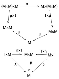
 is an arrow from
  , which we’ll call a multiplication operator.
 is an arrow from
  , called unit.
 is an arrow from
 \times M \rightarrow M \times (M\times M)") which represents the associativity property of the monoid.
which represents the associativity property of the monoid. ), and
 ") .
. \times M") composes with multiplication to be
composes with multiplication to be  .
.") .
.![A[\Gamma]](http://l.wordpress.com/latex.php?latex=A%5B%5CGamma%5D&bg=FFFFFF&fg=000000&s=0 "A[\Gamma]") , where A is a statement, and B is a set of assumptions. For example,
, where A is a statement, and B is a set of assumptions. For example, ![F(a) [a \in A, \Delta]](http://l.wordpress.com/latex.php?latex=F%28a%29%20%5Ba%20%5Cin%20A%2C%20%5CDelta%5D&bg=FFFFFF&fg=000000&s=0 "F(a) [a \in A, \Delta]") means that
means that ") is true, provided we’re in a context that includes
is true, provided we’re in a context that includes ![\frac{A \,\text{type}}{a \in A \,[a \in A]}](http://l.wordpress.com/latex.php?latex=%5Cfrac%7BA%20%5C%2C%5Ctext%7Btype%7D%7D%7Ba%20%5Cin%20A%20%5C%2C%5Ba%20%5Cin%20A%5D%7D&bg=FFFFFF&fg=000000&s=0 "\frac{A \,\text{type}}{a \in A \,[a \in A]}")
 is saying that
 ![\frac{a \in A \, []}{A \, \text{true}}](http://l.wordpress.com/latex.php?latex=%20%5Cfrac%7Ba%20%5Cin%20A%20%5C%2C%20%5B%5D%7D%7BA%20%5C%2C%20%5Ctext%7Btrue%7D%7D&bg=FFFFFF&fg=000000&s=0 "\frac{a \in A \, []}{A \, \text{true}}")


 in type
 ![C(x) \, \text{type} [x \in A]](http://l.wordpress.com/latex.php?latex=C%28x%29%20%5C%2C%20%5Ctext%7Btype%7D%20%5Bx%20%5Cin%20A%5D&bg=FFFFFF&fg=000000&s=0 "C(x) \, \text{type} [x \in A]") , which says that applying
, which says that applying ![\frac{C(x) \, \text{type} [x \in A] \quad a \in A}{C(a) \, \text{type}}](http://l.wordpress.com/latex.php?latex=%20%5Cfrac%7BC%28x%29%20%5C%2C%20%5Ctext%7Btype%7D%20%5Bx%20%5Cin%20A%5D%20%5Cquad%20a%20%5Cin%20A%7D%7BC%28a%29%20%5C%2C%20%5Ctext%7Btype%7D%7D&bg=FFFFFF&fg=000000&s=0 "\frac{C(x) \, \text{type} [x \in A] \quad a \in A}{C(a) \, \text{type}}")
") will be a type. In logical terms, it’s pretty straightforward; in programming terms it’s even clearer: if
will be a type. In logical terms, it’s pretty straightforward; in programming terms it’s even clearer: if ![\frac{C(x) \, \text{type}[x \in A] \quad a = b \in A}{C(a) = C(b)}](http://l.wordpress.com/latex.php?latex=%20%5Cfrac%7BC%28x%29%20%5C%2C%20%5Ctext%7Btype%7D%5Bx%20%5Cin%20A%5D%20%5Cquad%20a%20%3D%20b%20%5Cin%20A%7D%7BC%28a%29%20%3D%20C%28b%29%7D&bg=FFFFFF&fg=000000&s=0 "\frac{C(x) \, \text{type}[x \in A] \quad a = b \in A}{C(a) = C(b)}")
") isn’t quite a function. It’s a logical stamement which includes the symbol
isn’t quite a function. It’s a logical stamement which includes the symbol ![\frac{c(x) \in C(x) [x \in A] \quad a \in A}{c(a) \in C(A)}](http://l.wordpress.com/latex.php?latex=%20%5Cfrac%7Bc%28x%29%20%5Cin%20C%28x%29%20%5Bx%20%5Cin%20A%5D%20%5Cquad%20a%20%5Cin%20A%7D%7Bc%28a%29%20%5Cin%20C%28A%29%7D&bg=FFFFFF&fg=000000&s=0 "\frac{c(x) \in C(x) [x \in A] \quad a \in A}{c(a) \in C(A)}")
") is a proof-element: it’s an instance of
is a proof-element: it’s an instance of ") is a type, and we can see
is a type, and we can see  as a computation which, given an element of
 ") is an instance of type
is an instance of type ![\frac{c(x) \in C(x) [x \in A] \quad a = b}{c(a)=c(b)\in C(a)}](http://l.wordpress.com/latex.php?latex=%5Cfrac%7Bc%28x%29%20%5Cin%20C%28x%29%20%5Bx%20%5Cin%20A%5D%20%5Cquad%20a%20%3D%20b%7D%7Bc%28a%29%3Dc%28b%29%5Cin%20C%28a%29%7D&bg=FFFFFF&fg=000000&s=0 "\frac{c(x) \in C(x) [x \in A] \quad a = b}{c(a)=c(b)\in C(a)}")
") where:
where: is the number of inputs to the machine. We’ll represent a given input as a vector
 ![v=[v_1, ..., v_n]](http://l.wordpress.com/latex.php?latex=v%3D%5Bv_1%2C%20...%2C%20v_n%5D&bg=FFFFFF&fg=000000&s=0 "v=[v_1, ..., v_n]") .
.![\theta = [\theta_1, \theta_2, ..., \theta_n]](http://l.wordpress.com/latex.php?latex=%5Ctheta%20%3D%20%5B%5Ctheta_1%2C%20%5Ctheta_2%2C%20...%2C%20%5Ctheta_n%5D&bg=FFFFFF&fg=000000&s=0 "\theta = [\theta_1, \theta_2, ..., \theta_n]") is a vector of weights, where
is a vector of weights, where  is the weight for input
  .
. , the machine computes the combined, weighted input value
  by taking the dot product
 ![v \cdot w = [\theta_1v_1 + \theta_2v_2 + ... + \theta_nv_n]](http://l.wordpress.com/latex.php?latex=v%20%5Ccdot%20w%20%3D%20%5B%5Ctheta_1v_1%20%2B%20%5Ctheta_2v_2%20%2B%20...%20%2B%20%5Ctheta_nv_n%5D&bg=FFFFFF&fg=000000&s=0 "v \cdot w = [\theta_1v_1 + \theta_2v_2 + ... + \theta_nv_n]") . If
. If  , the neuron “fires” by producing a 1; otherwise, it produces a zero.
 that minimize the errors in assigning points to subspaces.
 + b")
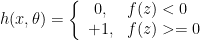
}") is the “true” value (that is, the correct classification) for value
is the “true” value (that is, the correct classification) for value }") is the value produced by the current set of weights of our perceptron. Then the
is the value produced by the current set of weights of our perceptron. Then the} - y^{(i)})^2")
}") is given to us with our training data.
is given to us with our training data.  , there’s a countour of a curve for all of the bindings that produce that level of error. All we need to do is follow the curve towards the minimum.
 called the learning rate.
}(t^{(i)} - y^{(i)})")
 on the set, with the additional property that for any subset
  ,
,  that you can define, describe, or compute,