
Paul Krugman has taken to calling certain kinds of economic ideas zombie economics, because no matter how many times they’re shown to be false, they just keep coming back from the dead. I certainly don’t have stature that compares in any way to Krugmant, but I’m still going to use his terminology for some bad math. There are some crackpot ideas that you just can’t kill.
For example, vortex math. I wrote about vortex math for the first time in 2012, again in early 2013, and again in late 2013. But like a zombie in a bad movie, it’s fans won’t let it stay dead. There must have been a discussion on some vortex-math fan forum recently, because over the last month, I’ve been getting comments on the old posts, and emails taking me to task for supposedly being unfair, closed-minded, ignorant, and generally a very nasty person.
Before I look at any of their criticisms, let’s start with a quick refresher. What is vortex math?
We’re going to create a pattern of single-digit numbers using multiples of 2. Take the number 1. Multiply it by 2, and you get 2. Multiple it by 2, and you get 4. Again, you get 8. Again, and you get 16. 16 is two digits, but we only want one-digit numbers, so we add them together, getting 7. Double, you get 14, so add the digits, and you get 5. Double, you get 10, add the digits, and you get 1. So you’ve got a repeating sequence: 1, 2, 4, 8, 7, 5, …

Take the numbers 1 through 9, and put them at equal distances around the perimeter of a circle. Draw an arrow from a number to its single-digit double. You end up with something that looks kinda-sorta like the infinity symbol. You can also fit those numbers onto the surface of a torus.

That’s really all there is to vortex math. This guy named Marco Rodin discovered that there’s a repeating pattern, and if you draw it on a circle, it looks kinda-like the infinity symbol, and that there must be something incredibly profound and important about it. Launching from there, he came up with numerous claims about what that means. According to vortex math, there’s something deeply significant about that pattern:
- If you make metallic windings on a toroidal surface according to that pattern and use it as a generator, it will generate free energy.
- Take that same coil, and run a current through it, and you have a perfect, reactionless space drive (called “the flux thruster atom pulsar electrical ventury space time implosion field generator coil”).
- If you use those numbers as a pattern in a medical device, it will cure cancer, as well as every other disease.
- If you use that numerical pattern, you can devise better compression algorithms that can compress any string of bits.
- and so on…
Essentially, according to vortex math, that repeated pattern of numbers defines a “vortex”, which is the deepest structure in the universe, and it’s the key to understanding all of math, all of physics, all of metaphysics, all of medicine. It’s the fundamental pattern of everything, and by understanding it, you can do absolutely anything.
As a math geek, the problem with stuff like vortex math is that it’s difficult to refute mathematically, because even though Rodin calls it math, there’s really no math to it. There’s a pattern, and therefore magic! Beyond the observation that there’s a pattern, there’s nothing but claims of things that must be true because there’s a pattern, without any actual mathematical argument.
Let me show you an example, from one of Rodin’s followers, named Randy Powell.
I call my discovery the ABHA Torus. It is now the full completion of how to engineer Marko Rodin’s Vortex Based Mathematics. The ABHA Torus as I have discovered it is the true and perfect Torus and it has the ability to reveal in 3-D space any and all mathematical/geometric relationships possible allowing it to essentially accomplish any desired functional application in the world of technology. This is because the ABHA Torus provides us a mathematical framework where the true secrets of numbers (qualitative relationships based on angle and ratio) are revealed in fullness.
This is why I believe that the ABHA Torus as I have calculated is the most powerful mathematical tool in existence because it presents proof that numbers are not just flat imaginary things. To the contrary, numbers are stationary vector interstices that are real and exhibiting at all times spatial, temporal, and volumetric qualities. Being stationary means that they are fixed constants. In the ABHA Torus the numbers never move but the functions move through the numbers modeling vibration and the underlying fractal circuitry that natures uses to harness living energy.
The ABHA Torus as revealed by the Rodin/Powell solution displays a perfectly symmetrical spin array of numbers (revealing even prime number symmetry), a feat that has baffled countless scientists and mathematicians throughout the ages. It even uncovers the secret of bilateral symmetry as actually being the result of a diagonal motion along the surface and through the internal volume of the torus in an expanding and contracting polarized logarithmic spiral diamond grain reticulation pattern produced by the interplay of a previously unobserved Positive Polarity Energetic Emanation (so-called ‘dark’ or ‘zero-point’ energy) and a resulting Negative Polarity Back Draft Counter Space (gravity).
If experimentally proven correct such a model would for example replace the standard approach to toroidal coils used in energy production today by precisely defining all the proportional and angular relationships existent in a moving system and revealing not only the true pathway that all accelerated motion seeks (be it an electron around the nucleus of an atom or water flowing down a drain) but in addition revealing this heretofore unobserved, undefined point energetic source underlying all space-time, motion, and vibration.
Lots of impressive sounding words, strung together in profound sounding ways, but what does it mean? Sure, gravity is a “back draft” of an unobserved “positive polarity energetic emanatation”, and therefore we’ve unified dark energy and gravity, and unified all of the forces of our universe. That sounds terrific, except that it doesn’t mean anything! How can you test that? What evidence would be consistent with it? What evidence would be inconsistent with it? No one can answer those questions, because none of it means anything.
As I’ve said lots of times before: there’s a reason for the formal framework of mathematics. There’s a reason for the painful process of mathematical proof. There’s a reason why mathematicians and scientists have devised an elaborate language and notation for expressing mathematical ideas. And that reason is because it’s easy to string together words in profound sounding ways. It’s easy to string together reasoning in ways that look like they might be compelling if you took the time to understand them. But to do actual mathematics or actual science, you need to do more that string together something that sounds good. You need to put together something that is precise. The point of mathematical notation and mathematical reasoning is to take complex ideas and turn them into precisely defined, unambiguous structures that have the same meaning to everyone who looks at them.
“positive polarity energetic emanation” is a bunch of gobbledegook wordage that doesn’t mean anything to anyone. I can’t refute the claim that gravity is a back-draft negative polarity energetic reaction to dark energy. I can’t support that claim, either. I can’t do much of anything with it, because Randy Powell hasn’t said anything meaningful. It’s vague and undefined in ways that make it impossible to reason about in any way.
And that’s the way that things go throughout all of vortex math. There’s this cute pattern, and it must mean something! Therefore… endless streams of words, without any actual mathematical, physical, or scientific argument.
There’s so much wrong with vortex math, but it all comes down to the fact that it takes some arbitrary artifacts of human culture, and assigns them deep, profound meaning for no reason.
There’s this pattern in the doubling of numbers and reducing them to one digit. Why multiple by two? Because we like it, and it produces a pretty pattern. Why not use 3? Well, because in base-10, it won’t produce a good pattern: [1, 3, 9, 9, 9, 9, ….] But we can pick another number like 7: [1, 7, 5, 8, 2, 5, 8, 2, 5, ….], and get a perfectly good series: why is that series less compelling than [1, 4, 8, 7, 2, 5]?
There’s nothing magical about base-10. We can do the same thing in base-8: [1, 2, 4, 1, 2, 4…] How about base-12, which was used for a lot of stuff in Egypt? [1, 2, 4, 8, 5, 10, 9, 7, 3, 6, 1] – that gives us a longer pattern! What makes base-10 special? Why does the base-10 pattern mean something that other bases, or other numerical representations, don’t? The vortex math folks can’t answer that. (Note: I made an arithmetic error in the initial version of the base-12 sequence above. It was pointed out in comments by David Wallace. Thanks!)
If we plot the numbers on a circle, we get something that looks kind-of like an infinity symbol! What does that mean? Why should the infinity symbal (which was invented in the 17th century, and chosen because it looked sort of like a number, and sort-of like the last letter of the greek alphabet) have any intrinsic meaning to the universe?
It’s giving profound meaning to arbitrary things, for unsupported reasons.
So what’s in the recent flood of criticism from the vortex math guys?
Well, there’s a lot of “You’re mean, so you’re wrong.” And there’s a lot of “Why don’t you prove that they’re wrong instead of making fun of them?”. And last but not least, there’s a lot of “Yeah, well, the fibonacci series is just a pattern of numbers too, but it’s really important”.
On the first: Yeah, fine, I’m mean. But I get pretty pissed at seeing people get screwed over by charlatans. The vortex math guys use this stuff to take money from “investors” based on their claims about producing limitless free energy, UFO space drives, and cancer cures. This isn’t abstract: this kind of nonsense hurts people. They people who are pushing these scams deserve to be mocked, without mercy. They don’t deserve kindness or respect, and they’re not going to get it from me.
I’d love to be proved wrong on this. One of my daughter’s friends is currently dying of cancer. I’d give up nearly anything to be able to stop her, and other children like her, from dying an awful death. If the vortex math folks could do anything for this poor kid, I would gladly grovel and humiliate myself at their feet. I would dedicate the rest of my life to nothing but helping them in their work.
But the fact is, when they talk about the miraculous things vortex math can do? At best, they’re delusional; more likely, they’re just lying. There is no cure for cancer in [1, 2, 4, 8, 7, 5, 1].
As for the Fibonacci series: well. It’s an interesting pattern. It does appear to show up in some interesting places in nature. But there are two really important differences.
- The Fibonacci series shows up in every numeric notation, in every number base, no matter how you do numbers.
- It does show up in nature. This is key: there’s more to it than just words and vague assertions. You can really find fragments of the Fibonacci series in nature. By doing a careful mathematical analysis, you can find the Fibonacci series in numerous places in mathematics, such as the solutions to a range of interesting dynamic optimization problems. When you find a way of observing the vortex math pattern in nature, or a way of producing actual numeric solutions for real problems, in a way that anyone can reproduce, I’ll happily give it another look.
- The Fibonacci series does appear in nature – but it’s also been used by numerous crackpots to make ridiculous assertions about how the world must work!
") where:
where: is the number of inputs to the machine. We’ll represent a given input as a vector
 ![v=[v_1, ..., v_n]](http://l.wordpress.com/latex.php?latex=v%3D%5Bv_1%2C%20...%2C%20v_n%5D&bg=FFFFFF&fg=000000&s=0 "v=[v_1, ..., v_n]") .
.![\theta = [\theta_1, \theta_2, ..., \theta_n]](http://l.wordpress.com/latex.php?latex=%5Ctheta%20%3D%20%5B%5Ctheta_1%2C%20%5Ctheta_2%2C%20...%2C%20%5Ctheta_n%5D&bg=FFFFFF&fg=000000&s=0 "\theta = [\theta_1, \theta_2, ..., \theta_n]") is a vector of weights, where
is a vector of weights, where  is the weight for input
  .
. is a bias value.
 is the threshold for firing.
 , the machine computes the combined, weighted input value
  by taking the dot product
 ![v \cdot w = [\theta_1v_1 + \theta_2v_2 + ... + \theta_nv_n]](http://l.wordpress.com/latex.php?latex=v%20%5Ccdot%20w%20%3D%20%5B%5Ctheta_1v_1%20%2B%20%5Ctheta_2v_2%20%2B%20...%20%2B%20%5Ctheta_nv_n%5D&bg=FFFFFF&fg=000000&s=0 "v \cdot w = [\theta_1v_1 + \theta_2v_2 + ... + \theta_nv_n]") . If
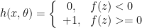
. If  , the neuron “fires” by producing a 1; otherwise, it produces a zero.
 :
:
 that minimize the errors in assigning points to subspaces.
 , we can define the operation of our more powerful in two phases. First, the perceptron computes the logit, which is the same old dot-product of the weights and the inputs. Then it applies the activation function to the logit, and based on the output, it decides whether or not to fire.
 + b")
}") is the “true” value (that is, the correct classification) for value
is the “true” value (that is, the correct classification) for value }") is the value produced by the current set of weights of our perceptron. Then the
is the value produced by the current set of weights of our perceptron. Then the} - y^{(i)})^2")
}") is given to us with our training data.
is given to us with our training data.  .
.  , there’s a countour of a curve for all of the bindings that produce that level of error. All we need to do is follow the curve towards the minimum.
 called the learning rate.
 above, we can expand that out to:
}(t^{(i)} - y^{(i)})")
 is well-ordered if there exists a total ordering
  on the set, with the additional property that for any subset
  ,
,  has a smallest element.
 that you can define, describe, or compute,
  % probability that the value for the full population lies within the margin of error of the measured value of the sample.”.
 ") up to isomorphism. To understand that, we’re implicitly referencing the formal definition of a field (with all of its sub-definitions) and the formal definitions of the addition, multiplication, and ordering operations.
up to isomorphism. To understand that, we’re implicitly referencing the formal definition of a field (with all of its sub-definitions) and the formal definitions of the addition, multiplication, and ordering operations.